Intermittency and the passive nature of the magnitude of the magnetic field

Abstract

It is shown that the statistical properties of the magnitude of the magnetic field in turbulent electrically conducting media resemble, in the inertial range, those of passive scalars in fully developed three-dimensional fluid turbulence. This conclusion, suggested by the data from Advanced Composition Explorer, is supported by a brief analysis of the appropriate magnetohydrodynamic equations.

In recent years, the problem of turbulent advection and diffusion of scalar and vector fields, both passive and active, has received renewed attention (see, for instance, Refs. shr -ching and the papers cited there). Corresponding experimental results are still few in number, partly because one is still grappling with the precise correspondence between the hypotheses of the theory and their experimental realization. We discuss here one of the most interesting examples considered recently: the case of magnetohydrodynamics (MHD) in which the magnetic field fluctuation ${\bf B}$ is described by the equation

$$\frac{\partial{\bf B}}{\partial t}=\nabla\times({\bf v}\times{\bf B})+\eta\nabla^{2}{\bf B}.$$

Here, ${\bf v}$ is the turbulence velocity and the $\eta$ is magnetic diffusivity. Equation (1) can be regarded as a vector analogue of the advection-diffusion equation

$$\frac{\partial\theta}{\partial t}=-({\bf v}\cdot\nabla)\theta+D\nabla^{2}\theta$$

for the evolution of a passive scalar $\theta$ subject to molecular diffusivity $D$. Aside from the fact that ${\bf B}$ is a vector and $\theta$ a scalar, the equations are different also because $\bf v$ in Eq. (1) can be affected quite readily by the feedback of the magnetic field $\bf B$. Our interest here is to explore the extent of similarities, despite these obvious differences, in the inertial range statistics of the magnetic and passive scalar fields.

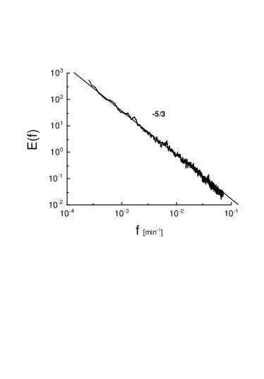
Figure 1: Energy spectrum of the magnitude $B=\sqrt{B_{i}^{2}}$ of the magnetic field $\bf B$ in the solar wind plasma, as measured by the ACE magnetometers in the nanoTesla range for the year 1998 (4 min average).

Solar wind is an excellent natural “laboratory” for the MHD problem. It is known that the statistical properties of velocity fluctuations in the solar wind are remarkably similar to those observed in fluid turbulence bur . It is also known that the plasma power spectra of the magnetic field and velocity fluctuations often contain an “inertial” range with a slope of approximately $-5/3$ (for reviews, see gold ,bur ). The approximately $-5/3$ power-law is especially common for magnitude fluctuations $B=\sqrt{B_{i}^{2}}$ (the summation over repeated indexes is assumed) of the magnetic field, as one can see in Fig. 1. For computing this spectrum, we have used the data obtained from Advanced Composition Explorer (ACE) satellite magnetometers for the year 1998. In this period, the sun was quiet and the data are statistically stable. The range of scales for which the “$-5/3$” power holds is taken to be the inertial range; the smaller scales are obliterated because of the instrument resolution and the truncation at the large-scale end is governed by the record length chosen for Fourier transforming.

The nature of the spectrum for each individual component of the magnetic field is more variable from one component of $\bf B$ to another, and from one situation to another, perhaps because of large anisotropies in the magnetic field $\bf B$, but the result for the $magnitude$ of $\bf B$ seems more robust. Scaling spectrum with the $-5/3$ slope (Fig. 1) is quite typical of that observed for passive scalar fluctuations in fully developed three-dimensional fluid turbulence (the so-called Corrsin-Obukhov spectrum my ). Spurred by this similarity, we were motivated to explore further the properties of the magnitude $B$, and compare them with those of the passive scalar. More detailed statistical information is provided by the structure functions scaling

$$\langle|\Delta B_{\tau}|^{p}\rangle\sim\tau^{\zeta_{p}},$$

where

$$\Delta B_{\tau}=B(t+\tau)-B(t).$$

The exponent $\zeta_{2}$ is directly related to the spectral exponent (in our case $\zeta_{2}\approx 5/3-1=2/3$ my ). If the dependence of $\zeta_{p}$ on $p$ is nonlinear, it is well-known that one has to deal with intermittency.

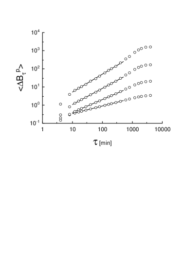
Figure 2: Structure functions of magnetic field magnitude in the solar wind plasma as measured by the ACE magnetometers in nanoTesla for the year 1998 (4 min averages). The straight lines (the best fits) are drawn to indicate the scaling law (3) in the inertial range.

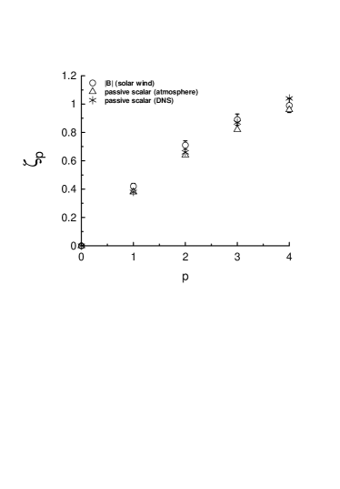
Figure 3: Scaling exponents (3) calculated for $B$ in the solar wind (circles) and for the passive scalar in the atmospheric turbulence (triangles, schmidt ), and in the direct numerical simulation of 3D fluid turbulence (stars, gotoh )

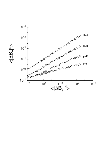
Figure 4: Extended self-similarity (ESS) of the magnetic field magnitude in the solar wind plasma. The straight lines (the best fit) are drawn to indicate the ESS (6).

Figure 5: The same as in Fig. 3 but using the ESS method (6) for $B$.

Figure 2 shows the scaling of structure functions for the solar wind data. Slopes of the straight-line fits in the apparently scaling region provide us the scaling exponents $\zeta_{p}$; these are shown in Fig. 3 as circles. Triangles in the figure indicate experimental values obtained for temperature fluctuations in the atmosphere schmidt . The other experimental data other1 ,other2 are in agreement with each other to better than 5$\%$. The $\star$ symbols are for the passive scalar field obtained by numerically solving the advection-diffusion in three-dimensional turbulence gotoh . It is clear that the exponents for the passive scalar data are in essential agreement with those for the magnitude fluctuations of the magnetic field.

One can, in fact, analyze the solar wind data somewhat differently using the notion of the extended self-similarity (ESS). Since, empirically, the fourth order exponent is quite closely equal to 1 for the magnetic field magnitude, i.e.,

$$\langle|\Delta B_{\tau}|^{4}\rangle\sim\tau,$$

we can extend the scaling range (and consequently improve the confidence with which those exponents are determined) by redefining them as

$$\langle|\Delta B_{\tau}|^{p}\rangle\sim\langle|\Delta B_{\tau}|^{4}\rangle^{\zeta_{p}}.$$

Figure 4 shows the ESS dependence (6). The slopes of the best-fit straight lines in this figure provide us with the ESS scaling exponents $\zeta_{p}$, which are shown in Fig. 5 as circles. The other symbols have remained unchanged from Fig. 3. The shift of the exponents $\zeta_{p}$ in comparison to those from ordinary self-similarity is about 4$\%$, but the scaling interval for ESS is considerably larger. This increased scaling range is well-known in other contexts ben .

The results shown in Figs. 3 and 5 suggest that at least up to the level of the fourth-order the scaling exponents for the passive scalars and for the magnitude of the magnetic field are essentially the same. This is both surprising and thought-provoking, and needs to be understood further. To this end, let us return to Eq. (1) and specialize comment , for simplicity, to the case of incompressible moving medium ($\nabla\cdot{\bf v}=0$). Equation (1) can then be rewritten as

$$\frac{\partial{\bf B}}{\partial t}=-({\bf v}\cdot\nabla){\bf B}+({\bf B}\cdot\nabla){\bf v}+\eta\nabla^{2}{\bf B}.$$

Let us now consider the equation for the magnitude $B$ of the magnetic fluctuations given by ${\bf B}=B{\bf n}$, where ${\bf n}$ is the unit vector with its direction along ${\bf B}$: $n_{i}=B_{i}/B$. Multiplying both sides of Eq. (7) by the vector ${\bf n}$ and taking into account that $n_{i}^{2}=1$ we obtain

$$\frac{\partial B}{\partial t}=-({\bf v}\cdot\nabla)B+\eta\nabla^{2}B+\lambda B,$$

in which the “friction-stretching” (or the production) coefficient $\lambda$ in the last term has the form

$$\lambda=n_{i}n_{j}\frac{\partial v_{i}}{\partial x_{j}}-\eta\left(\frac{\partial n_{i}}{\partial x_{j}}\right)^{2},$$

with the indices $i$ and $j$ representing the space coordinates, and the summation over repeated indexes is assumed. The first term on the right hand side of Eq. (9) is crucial for any dynamo effect.

If the statistical behaviors of $\theta$ and $B$ are to be similar, as suggested by Figs. 1, 3 and 5, we should be able to observe the underlying similarity between Eqs. (2) and (8). There is a major difference corresponding the presence in Eq. (8) of the production term $\lambda B$. However, given the empirical indications that $B$ and $\theta$ are similar in the inertial range, it is appropriate to look for circumstances under which the $\lambda$ term in Eq. (8) may be small. The second term in $\lambda$ is assured to be small because the smallness of the magnetic diffusivity $\eta$, but difficulties may arise from the first term on the right hand side of Eq. (9).

To eliminate directional dependencies in Eq. (8), let us make the following conditional average of that equation. That is, fix the magnitude $B$ in the vector field ${\bf B}=B{\bf n}$ while performing the average over all realizations of the direction vector field ${\bf n}$ permitted by the vector equation (7). Let us denote this ensemble average as $\langle...\rangle_{{\bf n}}$. From the definition, this averaging procedure does not affect $B$ itself, but affects the velocity field ${\bf v}$ and the “friction-stretching” coefficient $\lambda$ in Eq. (8). We thus obtain

$$\frac{\partial B}{\partial t}=-(\langle{\bf v}\rangle_{{\bf n}}\cdot\nabla)B+\eta\nabla^{2}B+\langle\lambda\rangle_{{\bf n}}B.$$

It is worth emphasizing that the solutions of the original equation (7) satisfy Eqs. (8) and (10), but not all possible formal solutions of the Eqs. (8) and (10) satisfy Eq. (7); similarly, not all formal solutions of Eq. (10) satisfy Eq. (8) while all solutions of Eq. (8) do satisfy Eq. (10). Restricting comments to the relationship between Eqs. (8) and (10), the solutions of the two equations are the same only if the initial conditions are the same and if realizations of $\langle{\bf v}\rangle_{\bf n}$ and of $\langle\lambda\rangle_{\bf n}$, related to these initial conditions by the conditional average procedure, are obtained from solutions applicable to Eq. (8).

Returning now to Eq. (10), the conditionally averaged velocity field $\langle{\bf v}\rangle_{{\bf n}}$ may posses statistical properties that are different from those of the original velocity field ${\bf v}$, and there can be circumstances under which $\langle\lambda\rangle_{{\bf n}}=0$, or small. If so, the similarity between Eqs. (2) and (10) (and, consequently, Eq. (8)) can be the basis for the similarity in statistical properties of their solutions. Therefore, finding conditions under which $\langle\lambda\rangle_{{\bf n}}=0$, or small, seems to be a useful exercise.

It is, however, difficult to guess a prioiri when $\langle\lambda\rangle_{{\bf n}}$ is negligible, because there is no small parameter for the stretching part of $\lambda$. Therefore, let us consider a generic set of conditions, presumably for the inertial range, which can result in $\langle n_{i}n_{j}\partial v_{i}/\partial x_{j}\rangle_{{\bf n}}=0$. This can be a combination of isotropy, which yields

$$\langle n_{i}n_{j}\rangle_{{\bf n}}=0~{}~{}~{}~{}(i\neq j)$$

and

$$\langle n_{1}^{2}\rangle_{{\bf n}}=\langle n_{2}^{2}\rangle_{{\bf n}}=\langle n_{3}^{2}\rangle_{{\bf n}},$$

and statistical independence

$$\langle n_{i}n_{j}\varphi\rangle_{{\bf n}}=\langle n_{i}n_{j}\rangle_{{\bf n}}\langle\varphi\rangle_{{\bf n}},$$

where $\varphi=\partial v_{k}/\partial x_{l}$ for arbitrary $k$ and $l$.

We should emphasize that the conditional average indicated by $\langle\dots\rangle_{{\bf n}}$ and the global average indicated by $\langle\dots\rangle$ are quite different; because of this, the quantity $B$ in (10) remains a fluctuating variable. To eliminate the stretching part from the conditionally averaged coefficient $\langle\lambda\rangle_{{\bf n}}$—this being critical for explaining the observed similarity in the scaling of structure functions between $B$ and $\theta$—one does not need to satisfy conditions (11) and (12) for all realizations of the magnetic field ${\bf B}$, but only for the subset of realizations that gives the main statistical contribution to the structure functions (3). Let us name this subset of realizations as I. The structure functions (3) depend on the statistical properties of the increments with respect to $\tau$, namely $\Delta B_{\tau}$, belonging to the inertial range of scales. One of the consequences of intermittency is that the statistical properties of the increments are essentially different from those of the field ${\bf B}$ itself. Therefore, the subset I need not generally coincide with the subset G, say, that gives the main statistical contribution to the global average $\langle n_{i}n_{j}\partial v_{k}/\partial x_{l}\rangle$. This means, in particular, that the conditions (11) and (12) can be valid for the inertial interval (i.e. for subset I), while globally (i.e. for subset G) these conditions could well be violated.

We now use conditions (11) and (12) in the presence of the incompressibility condition $\partial v_{i}/\partial x_{i}=0$ and obtain

$$\langle\lambda\rangle_{{\bf n}}=-\eta\langle\left(\frac{\partial n_{i}}{\partial x_{j}}\right)^{2}\rangle_{{\bf n}}.$$

That is, the difference between the passive scalar equation (2) and the conditionally averaged equation (10) for $B$ is reduced to pure “friction” with the friction coefficient given by (13). Equation (10) can then be reduced in Lagrangian variables to

$$\frac{dB}{dt}=\langle\lambda\rangle_{{\bf n}}B,$$

with the “multiplicative noise” $\langle\lambda\rangle_{{\bf n}}$ given by Eq. (13). Weak diffusion of Lagrangian “particles” can be described as their wandering around the deterministic trajectories. Introduction of a weak diffusion is equivalent to introduction of additional averaging in Eq. (14) over random trajectories zeld1 . The small parameter $\eta$ in (13) and (14) will then determine a slow time in comparison with the time scales in the inertial interval and will therefore not affect scaling properties of $B$ in the inertial interval. This explains the similarity of scaling between $B$ and $\theta$.

In summary, we have shown that remarkable scaling similarities exist in the inertial range between the passive scalar and the magnitude of the magnetic field in MHD flows. Motivated by this observation, we have derived the dynamical equation for $B$ and argued that, under circumstances governed by Eqs. (11) and (12), dynamical similarity exists between the equations governing the passive scalar and the magnitude of the magnetic fluctuations. The conditions under which (11) and (12) are valid, perhaps best described as “directional randomness”, may be quite general and applicable to other circumstances (though, perhaps, not for the vorticity equation whose form is strongly nonlinear in any turbulent situation).

We are grateful to ACE/MAG instrument team as well as to the ACE Science Center for providing the data and support, to T. Gotoh for providing Ref. gotoh before publication, and to G. Falkovich, to J. Schumacher and to V. Yakhot for comments.

References

- (1) B.I. Shraiman and E.D. Siggia, Nature 405, 639 (2000).
- (2) G. Falkovich, K. Gawedzki and M. Vergassola, Rev. Mod. Phys. 73, 913 (2001).
- (3) Y. Cohen, T. Gilbert and I. Procaccia, Phys. Rev. E 65, 026314 (2002).
- (4) E.S.C. Ching, Y. Cohen, T. Gilbert and I. Procaccia, Phys. Rev. E 67, 016304 (2003).
- (5) L. F. Burlaga, Interplanetary Magnetohydrodynamics (Oxford University Press, New York) 1995.
- (6) M.L. Goldstein, Astrophys. Space Sci. 227, 349 (2001)
- (7) A.S. Monin and A.M. Yaglom, Statistical Fluid Mechanics: Mechanics of Turbulence, vol. 2 (MIT Press, Cambridge) 1975.
- (8) F. Schmitt, D. Schertzer, S. Lovejoy and Y. Brunet, Europhys. Lett. 34, 195 (1996).
- (9) T. Watanabe and T. Gotoh, Statistics of Passive Scalar in Homogeneous Turbulence (submitted).
- (10) R.A. Antonia, E. Hopfinger, Y. Gagne and F. Anselmet, Phy. Rev. A 30, 2705 (1984).
- (11) C. Meneveau, K.R. Sreenivasan, P. Kailasnath and M.S. Fan, Phys. Rev. A 41, 894 (1990).
- (12) R. Benzi, L. Biferale, S. Ciliberto, M.V. Struglia and R. Tripiccione, Physica D 96, 162 (1996).
- (13) This is not overly restrictive in the inertial range; see, e.g., M.L. Goldstein, D.A. Roberts and W.H. Matthaeus, Annu. Rev. Astron. Astrophys. 33, 283 (1995).
- (14) Ya.B. Zeldovich, A.A. Ruzmaikin and D.D. Sokoloff, Magnetic Fields in Astrophysics (Gordon and Breach) 1983; Ya.B. Zeldovich, B. Molchanov, A.A. Ruzmaikin, D.D. Sokolov Sov. Phys. Usp. 30, 353 (1987).