Soliton Lattice and Single Soliton Solutions of the Associated Lamé and Lamé Potentials

Abstract

We obtain the exact nontopological soliton lattice solutions of the Associated Lamé equation in different parameter regimes and compute the corresponding energy for each of these solutions. We show that in specific limits these solutions give rise to nontopological (pulse-like) single solitons, as well as to different types of topological (kink-like) single soliton solutions of the Associated Lamé equation. Following Manton, we also compute, as an illustration, the asymptotic interaction energy between these soliton solutions in one particular case. Finally, in specific limits, we deduce the soliton lattices, as well as the topological single soliton solutions of the Lamé equation, and also the sine-Gordon soliton solution.

I Introduction

Over the years, extensive research has been carried out seeking the exact soliton solutions of both periodic (e.g., sine-Gordon, double sine-Gordon) and nonperiodic (e.g., $\phi^{4}$, $\phi^{6}$) field theory models. For example, the exactly solvable sine-Gordon (SG) equation sg and its quasi-exactly solvable (QES) partner, i.e., the double sine-Gordon equation (DSG), have exact single soliton leung ; peyrard as well as soliton lattice dando solutions.

There have been some advances in the study of the hyperbolic analogues of these problems; the exactly solvable hyperbolic analogue of the SG equation is the sine-hyperbolic Gordon (ShG) equation shg . This potential has only one minimum and thus does not support (topological) soliton solutions. The hyperbolic analogue of the DSG equation is the double sine-hyperbolic Gordon (DShG) equation, which is a QES double-well potential with exact single soliton and soliton lattice solutions dshg .

However, not much is known regarding the elliptic analogues of these problems. The elliptic ‘generalization’ of the SG is the Lamé equation arscott but, as far as we are aware of, its single soliton and soliton lattice solutions have not been worked out yet. One would surmise that the elliptic analogue of the DSG equation is the Associated Lamé (AL) equation magnus ; khare ; ganguly . Nevertheless, we find below that this is not the case.

Generally speaking, the Schrödinger equations with periodic potentials belong to a class known as Hill’s equations magnus , and they lead to a band structure of the energy spectrum of the system. For both the SG and DShG potentials one could calculate the exact statistical and thermodynamical properties dshg ; gupta through a knowledge of the spectral band structure and their solitonic and phononic solutions, respectively. Both AL and Lamé are also periodic potentials with a band structure arscott ; khare ; ganguly . Although our goal in the present paper is only to obtain their exact single soliton and soliton lattice solutions, this will serve as a background for future statistical mechanics studies of the AL and Lamé elliptic potentials. In particular, we obtain here the soliton lattice solutions of the AL equation in different parameter regimes corresponding to different shapes of the AL potential. The advantage of this approach is that the corresponding single pulse and topological soliton solutions of the AL equation can be immediately obtained from the lattice solution in suitable limits. Furthermore, the soliton lattices and topological single soliton solutions of the Lamé equation are easily obtained by taking a different appropriate limit. Besides, the asymptotic interaction between the solitons can also be readily obtained by using Manton’s formalism manton .

Our results can be summarized as follows: We show that there are six different soliton lattice solutions of the AL equation for different values of the parameters. From these six solutions we obtain the corresponding AL single soliton solutions. It turns out that while in five cases these are topological (kink-like) single solitons, in one case we have a nontopological (pulse-like) single soliton solution. From the AL soliton lattice solutions, by taking appropriate limits, we also obtain the corresponding Lamé soliton lattices and single soliton solutions.

There are many physical contexts in which the Lamé equation arises, such as bond-order and charge density wave systems horovitz , nonlinear elasticity zhurav , and other contexts, e.g., phase slips in superconductors and magnetoelastic interaction on curved surfaces. The AL equation could arise in the above systems in the presence of external – electric, magnetic or stress – fields.

The plan of the paper is as follows. In Sec. II we discuss some salient features of the AL potential. In Sec. III we obtain the nontopological soliton lattice solutions of the AL equation in different regimes in the parameter space and also compute the corresponding energies. In Sec. IV we obtain the topological and pulse single soliton solutions of the AL equation by taking the appropriate limits of the various nontopological solutions obtained in the previous section. It is worth emphasizing here that in one special case, we obtain two different kinds of topological solutions of the AL equation. As an illustration, in one particular case, we also estimate the asymptotic interaction between these single solitons. (In all the other cases one can follow exactly the same procedure, and thus we will not consider these here.) As a crosscheck on our results, we recover in appropriate limit, the sine-Gordon soliton solution. In Sec. V we show that by taking an appropriate limit, we can also obtain the kink lattice and the topological single soliton solutions of the Lamé equation. Finally, in Sec. VI we summarize the results obtained in this paper and indicate some open problems.

II The Associated Lamé potential

Consider the following family of periodic potentials labeled by a pair of real parameters $(p,\,q)$:

$$V_{AL}(\phi,\,k)\,=\,p\,k^{2}\,\mbox{sn}^{2}(\phi,\,k)\,+\,q\,k^{2}\,\displaystyle\frac{\mbox{cn}^{2}(\phi,\,k)}{\mbox{dn}^{2}(\phi,\,k)}\,+\,C\,=\,p\,k^{2}\,\mbox{sn}^{2}(\phi,\,k)\,+\,q\,k^{2}\,\displaystyle{\mbox{sn}^{2}(\phi+K(k),\,k)}\,+\,C~{},$$ (1)

that are called Associated Lamé potentials (since the corresponding Schrödinger equation is called the Associated Lamé equation) magnus ; khare ; ganguly . Here $\mbox{sn}(\phi,\,k)$ and $\mbox{cn}(\phi,\,k)$ are respectively the sine and cosine amplitude Jacobi elliptic functions of real modulus $k$ ($0\,\leqslant\,k\,\leqslant 1$) and period $4\,K(k)$; $\mbox{dn}(\phi,\,k)$ is the $\delta$-amplitude Jacobi elliptic function of modulus $k$ and period $2\,K(k)$; and $K(k)$ denotes the complete elliptic integral of the first kind, see gradshteyn ; byrd . We will choose the constant $C$ in the potential so that the absolute minimum of the potential–with respect to $\phi$–equals zero, $V_{min}\,=\,0$. The potential is periodic with period $2K(k)$, except in the limit $p=q$ when the period reduces to K(k), as it is clear from Eq. (1).

The case $q\,=\,0$ corresponds to the standard Lamé potential $V_{L}(\phi,\,k)$. There are two more cases in which the potential (1) reduces to the Lamé potential. Namely, when $p\,=\,0$ and also when $p\,=\,q$, as shown below. Therefore in all the calculations below we will admit that $p\,\neq\,0$ and $p\,\neq\,q$; the results for the standard Lamé potential will be recovered in the limit $q\,\rightarrow 0$, and we refer to these results whenever the potential reduces to the standard Lamé one. From a physical point of view, if one thinks of a Lamé potential $(p,0)$ as due to a one-dimensional array of atoms with spacing $2K(k)$ and ‘strength’ $p$, then the Associated Lamé potential $(p,q)$ results from two alternating types of atoms spaced by $K(k)$ with ‘strengths’ $p$ and $q$, respectively. If the two types of atoms are identical (which makes $p~{}=~{}q$), one expects a potential of period $K(k)$.

In addition, when $k\,\rightarrow\,0$, and $|p|,\,|q|\,\rightarrow\infty$, so that $|p|\,k^{2}\,\rightarrow\,P$ = finite and $|q|\,k^{2}\,\rightarrow\,Q$ = finite, the potential (1) reduces to the sine-Gordon potential,

$$V_{sG}\,=\,(P\;\mbox{sign}\;p\,-\,Q\;\mbox{sign}\;{q})\,\sin^{2}\phi\,,$$ (2)

and the results we present below reduce to the well-known ones for the sine-Gordon potential.

It is also worth noting that under the transformation $\phi\rightarrow\phi+K(k)$ the AL potential (1) $V_{AL}(p,q)$ goes over into $V_{AL}(q,p)$ and hence for $p>0,q\geq 0$, as well as for $p<0,q\leq 0$, without loss of generality, we shall always consider the case of $p^{2}>q^{2}$. Further, instead of considering both the possibilities of $p>0,q\leq 0$ and $p<0,q\geq 0$, it suffices to consider just the case of $p>0,q\leq 0$, but now $p^{2}$ can be bigger as well as smaller than $q^{2}$.

Finally, consider the case of $p=q$, when, by using the Landen transform gradshteyn and choosing the constant $C=-pk^{2}$, the AL potential (1) can be written as

$$V_{AL}(\phi,k)=(1-k^{\prime})^{2}V_{L}\left[(1+k^{\prime})\phi,\frac{1-k^{\prime}}{1+k^{\prime}}\right]~{},$$ (3)

where $k^{\prime}=\sqrt{1-k^{2}}$ is the complementary elliptic modulus. For the rescaled field $\tilde{\phi}=(1+k^{\prime})\phi$ and in the rescaled space coordinate $\tilde{x}=(1+k^{\prime})x$ the field equations [see next section, Eq. (5)] will remain the same as that for the simple Lamé potential. Note that the $p=q$ case cannot be obtained as a limit of $q\rightarrow p$ ($q\neq p$), since–as already mentioned–when $p=q$ the periodicity of the potential (1) is $K(k)$, while for $p\neq q$ it is $2\,K(k)$, see also khare .

III Soliton Lattice Solutions of the AL Potential

For the scalar field $\phi\,=\,\phi(x,\,t)$ the dynamics is described by the second-order hyperbolic differential equation

$$\frac{\partial^{2}\phi}{\partial t^{2}}\,-\,\displaystyle\frac{\partial^{2}\phi}{\partial x^{2}}\,=\,-\,\displaystyle\frac{\partial V_{AL}}{\partial\phi}\,.$$ (4)

In the stationary case $\phi\,=\,\phi(x)$, this reduces simply to

$$\frac{d^{2}\phi}{dx^{2}}\,=\,\displaystyle\frac{\partial V_{AL}}{\partial\phi}\,,$$ (5)

that can be easily integrated, at least formally, by quadratures. The time-dependent solutions are immediately obtained from here by Lorentz boosting. The physically meaningful solutions (bounded at $x\,\rightarrow\,\pm\,\infty$) are given by

$$\pm\,\sqrt{2}\,(x\,-\,x_{0})\,=\,\displaystyle\int_{\displaystyle\phi(x_{0})}^{\displaystyle\phi(x)}\displaystyle\frac{d\tilde{\phi}}{\sqrt{V_{AL}(\tilde{\phi},\,k)\,-\,A^{2}}}\,,$$ (6)

where $x_{0}$ and $A^{2}\equiv|p|\,k^{2}\,a^{2}$ are the two (suitably chosen) integration constants. Of course, $V_{min}\,=\,0\leqslant\,A^{2}\,<\,V_{max}$, where $V_{min/max}$ is the absolute minimum/maximum of the potential energy with respect to $\phi$. In fact, in view of the condition $V_{AL}(\tilde{\phi},\,k)\,-\,A^{2}\geqslant 0$, the actual value of $A^{2}$ determines the appropriate integration domain in Eq. (6).

Depending on the values of the parameters $p$ and $q$, the potential $V_{AL}(\phi,k)$ has different behaviors in one period $0\,\leqslant\,\phi\,<\,2\,K(k)$, and hence the nature of the solutions in Eq. (6) is also different. There are three cases to be considered separately, namely (I) when $p\,>\,0$ and $q\,\geqslant\,0$, (II) when $p\,<\,0$ and $q\,\leqslant\,0$, and, finally, (III) when $p\,>\,0$ and $q\,\leqslant\,0$. Note that in what follows we shall use the shorthand notation $\Gamma\,\equiv\,\sqrt{|{q}|/|{p}|}$.

III.1 Case I : $p\,>\,0$ and $q\,\geqslant\,0$

As explained above, in this case it is sufficient to consider $0\,\leqslant\,\Gamma\,<\,1$. Note that the case $\Gamma\,=\,0$ corresponds to the standard Lamé potential. Depending on the value of $\Gamma$, the potential $V_{AL}(\phi,\,k)$ can have different behaviors in one period $0\,\leqslant\,\phi\,<\,2\,K(k)$.

Case I.1 : $0\,\leqslant\,\Gamma\,\leqslant\,k^{\prime}$

Here $0\,\leqslant\,k^{\prime}\,=\,\sqrt{1\,-\,k^{2}}\,\leqslant\,1$ is the complementary elliptic modulus. The potential $V_{AL}(\phi)$ has only one minimum, $V_{min}\,=\,0$ (at $\phi\,=\,0$), and one maximum, $V_{max}\,=\,p\,k^{2}\,(1\,-\,\Gamma^{2})$ [at $\phi\,=\,K(k)$], in one period [note that we have chosen $C\,=\,-\,p\,k^{2}\,\Gamma^{2}$ in Eq. (1) in order to have $V_{min}=0$]. The plot of the potential $V_{AL}$ as a function of $\phi$ is given in Fig. 1(a), where the solid and the dashed horizontal lines correspond to two choices of the parameter $A^{2}$. Under the change of variable $\tilde{z}\,=\,\mbox{sn}^{2}(\tilde{\phi},\,k)$, Eq. (6) can be rewritten as

$$2\,\sqrt{2\,p\,k^{4}}\,x\,=\,\pm\,\displaystyle\int_{\displaystyle z}^{\displaystyle 1}\,\displaystyle\frac{d\tilde{z}}{\sqrt{(z_{1}\,-\,\tilde{z})\,(1\,-\,\tilde{z})\,(\tilde{z}\,-\,z_{2})\,(\tilde{z}\,-\,0)}}\,,$$ (7)

where $z=\mbox{sn}^{2}(\phi,\,k)$, $x_{0}\,=\,0$ for $\phi_{0}\,=\,K(k)$ (by choice) and $A^{2}\,=\,p\,k^{2}\,a^{2}$ with $0\,\leqslant a^{2}\,<\,(1\,-\,\Gamma^{2})$. The value of $a^{2}$ determines the limits of the integration interval in the above equation, through the condition $V(\phi_{1,2})\,-\,p\,k^{2}\,a^{2}\,=\,0$; one finds that $z_{1,2}\,=\,\mbox{sn}^{2}(\phi_{1,2})$ are given by:

$$z_{1,\,2}\,=\,\displaystyle\frac{1\,-\,\Gamma^{2}\,k^{{}^{\prime}2}\,+\,a^{2}\,k^{2}}{2\,k^{2}}\,\left[1\,\pm\,\sqrt{1\,-\,\displaystyle\frac{4\,k^{2}\,a^{2}}{(1\,-\,\Gamma^{2}\,k^{{}^{\prime}2}\,+\,a^{2}\,k^{2})^{2}}}\;\right]\,,$$ (8)

and $z_{1}\,>\,1\,>\,z\,\geqslant\,z_{2}\,>\,0$. Then the integral in (7) can be evaluated using the formula 3.147(5) of gradshteyn and one is finally led to the nontopological soliton lattice solution

$$\mbox{sn}^{2}(\phi,\,k) = \displaystyle\frac{[(z_{1}\,-\,z_{2})\,-\,z_{1}\,(1\,-\,z_{2})\,\mbox{sn}^{2}(y,\,t)]}{[(z_{1}\,-\,z_{2})\,-\,(1\,-\,z_{2})\,\mbox{sn}^{2}(y,\,t)]}\,.$$ (9)

Here $y\,=\,\sqrt{2\,p\,k^{4}\,(z_{1}\,-\,z_{2})}\;x$ and the period of the lattice $2\,L\,=\,2\,K(t)/\sqrt{2\,p\,k^{4}\,(z_{1}\,-\,z_{2})}$ is controlled by the modulus

$$0\,<\,t\,=\,\left[\displaystyle\frac{z_{1}\,(1\,-\,z_{2})}{z_{1}\,-\,z_{2}}\right]^{1/2}\,\leqslant\,1.$$ (10)

Note that $\phi$ oscillates between $K(k)$ and $\mbox{sn}^{-1}(\sqrt{z_{2}})$ [respectively, $-\,K(k)$ and $-\,\mbox{sn}^{-1}(\sqrt{z_{2}})$], i.e., it is indeed a nontopological solution [it does not connect two adjacent degenerate minima of the potential, that are separated by a distance–in the $\phi$ space–of $2\,K(k)$]. In Fig. 1(b) we give a plot of the solution (i.e., the field $\phi$ as a function of $x$) with solid and dashed curves corresponding to the two choices of $A^{2}$ as in Fig. 1(a), while the dotted curve represents the topological single soliton solution (corresponding to $A^{2}=0$)–see Sec. IV. We also note that there are no “cusps” in the actual profiles of the fields; indeed, in Fig. 1(b) and in the subsequent figures we have plotted modulo $2K(k)$ the absolute value of the actual field $\phi(x)$. Specifically, for solutions that touch $K(k)$ such as in Fig. 1(b), the actual field is $\phi(x)$ in $[0,2L]$, $2K(k)-\phi(x)$ in $[2L,4L]$, $\phi(x)$ in $[4L,6L]$, and so on. Similarly, for solutions that touch $0$ field value such as in Fig. 3(b), the actual field is $\phi(x)$ in $[0,2L]$, $-\phi(x)$ in $[2L,4L]$, $\phi(x)$ in $[4L,6L]$, and so on.

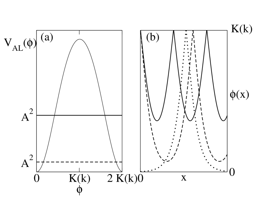
Figure 1: Case I.1 : $0\,\leqslant\,\Gamma\,\leqslant\,k^{\prime}$. (a) The shape of the potential $V_{AL}(\phi)$. The solid and the dashed horizontal lines correspond to two choices of the integration parameter $A^{2}$. (b) The soliton lattice solution [i.e., the field $\phi(x)$] with solid and dashed curves corresponding to the two values of $A^{2}$ in (a). The $x$-axis is not labeled because the two lattices have different spatial periods. The dotted curve represents the topological single soliton solution corresponding to $A^{2}=0$ (for the sake of clarity we have displaced the origin of the $x$-axis for this curve).

One can compute the energy corresponding to a period $2\,L$ of this soliton lattice:

$$E_{SL} = \displaystyle\int_{\displaystyle-\,L}^{\displaystyle L}\,\left[\frac{1}{2}\;\left(\frac{d^{2}\,\phi}{dx^{2}}\right)\,+\,V_{AL}(\phi)\right]\,dx\,=\,\int_{\displaystyle-\,L}^{\displaystyle L}\,\left[2\,V_{AL}(\phi)\,-\,A^{2}\right]\,dx\,$$ (11)

$$= \,4\,\int_{\displaystyle 0}^{\displaystyle L}V_{AL}(\phi)\,dx\,-2\,L\,A^{2}=4\,p\,k^{2}\,\int_{\displaystyle 0}^{\displaystyle L}\,\mbox{sn}^{2}[\phi(x),\,k]\,dx\,$$

$$+ \,4\,p^{2}\,k^{2}\,\Gamma^{2}\,\int_{\displaystyle 0}^{\displaystyle L}\left\{\displaystyle\frac{\mbox{cn}^{2}[\phi(x),\,k]}{\mbox{dn}^{2}[\phi(x),\,k]}\,-\,1\right\}\,dx\,-\,2\,L\,p^{2}\,k^{2}\,a^{2}\,.$$

After some algebraic manipulations, using the solution (9) one obtains:

$$E_{SL} = 2\,\sqrt{\displaystyle\frac{2\,p}{z_{1}\,-\,z_{2}}}\,\left\{\left[z_{1}\,K(t)\,-\,(z_{1}\,-\,1)\,\Pi\left(\displaystyle\frac{1\,-\,z_{2}}{z_{1}\,-\,z_{2}},\,t\right)\right]\,-\,\displaystyle\frac{a^{2}\,K(t)}{2}\right\}\,-\,$$ (12)

$$-\,\Gamma^{2}\,\left[\displaystyle\frac{z_{1}\,k^{{}^{\prime}2}}{1\,-\,z_{1}\,k^{2}}\,K(t)\,-\,\displaystyle\frac{z_{1}\,-\,1}{1\,-\,z_{1}\,k^{2}}\,\Pi\left(\displaystyle\frac{(1\,-\,z_{2})\,(1\,-\,z_{1}\,k^{2})}{(z_{1}\,-\,z_{2})\,k^{{}^{\prime}2}},\,t\right)\right]\,,$$

where $\Pi(z_{0},t)$ denotes the complete elliptic integral of the third kind gradshteyn ; byrd .

Case I.2 : $k^{\prime}\,<\,\Gamma\,<\,1$

The potential $V_{AL}(\phi)$ has now two minima: $V_{min}(\phi\,=\,0)\,=\,0$ and a local minimum $V^{l}_{min}[\phi\,=\,K(k)]\,=\,p\,k^{2}\,(1\,-\,\Gamma^{2})$, and two symmetric maxima around $\phi~{}=~{}K(k)$, namely $V_{max}\,=\,p\,k^{2}\,[(1\,-\,\Gamma\,k^{\prime})/k]^{2}$ for $\phi\,=\,\mbox{sn}^{-1}\left[\sqrt{(1\,-\,\Gamma\,k^{\prime})/k^{2}}\right],\,2\,K(k)\,-\,\mbox{sn}^{-1}\left[\sqrt{(1\,-\,\Gamma\,k^{\prime})/k^{2}}\right]$. The plot of the potential $V_{AL}(\phi)$ as a function of $\phi$ is given in Fig. 2(a), where the solid and the dashed horizontal lines correspond to the two choices of the integration constant $A^{2}$ as explained below. Note that in this case it makes no sense to consider either the limit of the Lamé potential (i.e., $\Gamma\,\rightarrow\,0$), or that of the sine-Gordon potential (i.e., $k\,\rightarrow\,0$, $p\,k^{2}\,\rightarrow\,P,\;q\,k^{2}\,\rightarrow\,Q$). There are two possible situations, depending on the value of $A^{2}=p\,k^{2}\,a^{2}$.

Case I.2(i) : $V_{min}\,\leqslant\,A^{2}=p\,k^{2}\,a^{2}\,<\,V^{l}_{min}$, i.e., $0\,\leqslant a^{2}\,<\,1\,-\,\Gamma^{2}$.
One recovers the same soliton lattice solution as above, Eq. (9), with the same modulus $t$, Eq. (10), and the same energy per period of the lattice, Eq. (12).

Case I.2(ii) : $V^{l}_{min}\,\leqslant\,A^{2}=p\,k^{2}\,a^{2}\,<\,V_{max}$, i.e., $1\,-\,\Gamma^{2}\,\leqslant\,a^{2}\,<\,[(1\,-\,\Gamma\,k^{\prime})/k]^{2}$.
Then the integral (6) becomes

$$2\,\sqrt{2\,p\,k^{4}}\,x\,=\,\pm\,\displaystyle\int_{\displaystyle z_{2}}^{\displaystyle z}\,\displaystyle\frac{d\tilde{z}}{\sqrt{(1\,-\,\tilde{z})\,(z_{1}\,-\,\tilde{z})\,(\tilde{z}\,-\,z_{2})\,(\tilde{z}\,-\,0)}}\,,$$ (13)

with $z\,=\,\mbox{sn}^{2}(\phi,\,k)$ and $1\,>\,z_{1}\,\geqslant\,z\,>\,z_{2}$ [$z_{1,2}$ have the same expressions as above, Eq. (8)]. One can evaluate this integral using the formula 3.147(4) of gradshteyn and obtain the following nontopological soliton lattice solution

$$\mbox{sn}^{2}(\phi,\,k)\,=\,\displaystyle\frac{z_{1}\,z_{2}}{z_{1}\,-\,(z_{1}\,-\,z_{2})\,\mbox{sn}^{2}(w,\,n)}\,,$$ (14)

with $w\,=\,\sqrt{2\,p\,k^{4}\,z_{1}\,(1\,-\,z_{2})}\;x$, and the modulus $n$ given by

$$0\,<\,n\,=\,\sqrt{\displaystyle\frac{z_{1}\,-\,z_{2}}{z_{1}\,(1\,-\,z_{2})}}\,\leqslant\,1\,;$$ (15)

therefore, the soliton lattice has a spatial period $2\,L\,=\,2\,K(n)/\sqrt{2\,p\,k^{4}\,z_{1}\,(1\,-\,z_{2})}$. Note that $\phi$ varies between $\mbox{sn}^{-1}(\sqrt{z_{1}})$ and $\mbox{sn}^{-1}(\sqrt{z_{2}})$ [respectively, $-\,\mbox{sn}^{-1}(\sqrt{z_{1}})$ and $-\,\mbox{sn}^{-1}(\sqrt{z_{2}})$] when $x$ varies over one spatial period: indeed, this solution is nontopological.

In Case I.2(ii) in order to compute the energy for one spatial period $2\,L$, it is useful to shift the potential by $-\,V^{l}_{min}\,=\,-\,p\,k^{2}\,(1\,-\,\Gamma^{2})$, so that the minimum of the potential explored by the soliton lattice is equal to zero. One finds:

$$E_{SL}=4\,\displaystyle\int_{\displaystyle 0}^{\displaystyle L}V_{AL}(\phi)\,dx\,-\,2\,L\,V^{l}_{min}\,-\,2\,L\,p^{2}\,k^{2}\,a^{2}\,=\,2\,\sqrt{\displaystyle\frac{2\,p^{2}}{z_{1}\,(1\,-\,z_{2})}}\,$$

$$\times\,\left[z_{2}\,\Pi\left(\displaystyle\frac{z_{1}\,-\,z_{2}}{z_{1}},\,n\right)\,-\,\Gamma^{2}\,\displaystyle\frac{k^{{}^{\prime}2}\,z_{2}}{1\,-\,k^{2}\,z_{2}}\,\Pi\left(\displaystyle\frac{z_{1}\,-\,z_{2}}{z_{1}\,(1\,-\,k^{2}\,z_{2})},\,n\right)\,-\,\displaystyle\frac{a^{2}\,+\,(1\,-\,\Gamma^{2})}{2}\right]\,.$$

(16)

The plot of the solutions in Case I.2 is given in Fig. 2(b), where the solid line corresponds to the nontopological soliton lattice solution of Case I.2(i), while the dashed line corresponds to the nontopological soliton lattice solution of Case I.2(ii). Note that in the appropriate limits (see Sec. IV) these two types of solutions give birth to a topological [Case I.2(i)] and a nontopological single soliton [Case I.2(ii)] solution, respectively.

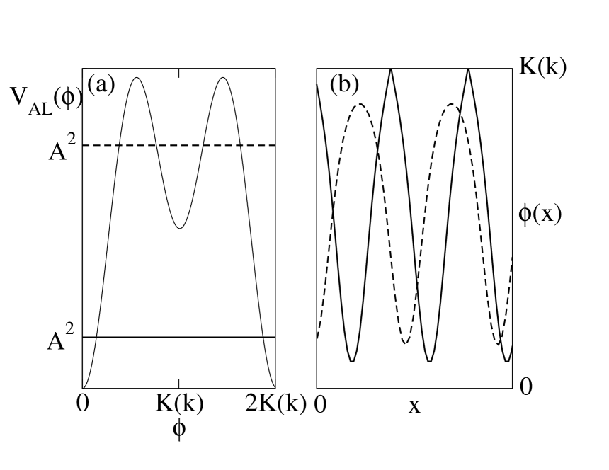
Figure 2: Case I.2 : $k^{\prime}\,<\,\Gamma\,<\,1$. (a) The shape of the potential $V_{AL}(\phi)$. The solid and the dashed horizontal lines correspond to two choices of the integration parameter $A^{2}$, namely, Case I.2(i) : $V_{min}\,\leqslant\,A^{2}=p\,k^{2}\,a^{2}\,<\,V^{l}_{min}$, i.e., $0\,\leqslant a^{2}\,<\,1\,-\,\Gamma^{2}$ (solid line); and Case I.2(ii) : $V^{l}_{min}\,\leqslant\,A^{2}=p\,k^{2}\,a^{2}\,<\,V_{max}$, i.e., $1\,-\,\Gamma^{2}\,\leqslant\,a^{2}\,<\,[(1\,-\,\Gamma\,k^{\prime})/k]^{2}$ (dashed line). (b) The soliton lattice solution [i.e., the field $\phi(x)$] with solid and dashed curves corresponding to the two values of $A^{2}$ in (a), i.e., respectively, to Case I.2(i) and Case I.2(ii). The $x$-axis is not labeled because the two lattices have different periodicities.

III.2 Case II : $p\,<\,0$ and $q\,\leqslant\,0$

As explained above, here again it suffices to focus only on the domain $0\,\leqslant\,\Gamma\,<\,1$, and we must distinguish between two different behaviors of the potential, depending on the value of $\Gamma$.

Case II.1 : $0\,\leqslant\,\Gamma\,\leqslant\,k^{\prime}$

The potential $V_{AL}(\phi,\,k)$ has only two extrema in $[0,\,2\,K(k))$, namely an absolute maximum $V_{max}\,=\,|p|\,k^{2}\,(1\,-\,\Gamma^{2})$ for $\phi\,=\,0$, and an absolute minimum $V_{min}\,=\,0$ for $\phi\,=\,K(k)$ [with the choice of the shift $C\,=\,|p|\,k^{2}$ in Eq. (1)]. A plot of the potential is given in Fig. 3(a).

One can repeat the integration scheme described in the preceding case. In particular, considering $z\,=\,\mbox{sn}^{2}(\phi,\,k)$, Eq. (6) becomes:

$$2\,\sqrt{2\,|p|\,k^{4}}\;x\,=\,\pm\,\int_{\displaystyle 0}^{\displaystyle z}\displaystyle\frac{d\tilde{z}}{\sqrt{(z_{1}\,-\,\tilde{z})\,(1\,-\,\tilde{z})\,(z_{2}\,-\,\tilde{z})\,(\tilde{z}\,-\,0)}}\,,$$ (17)

where this time

$$z_{1,\,2}\,=\,\displaystyle\frac{1\,+\,k^{2}\,-\,\Gamma^{2}\,-\,a^{2}\,k^{2}}{2\,k^{2}}\,\left[1\,\pm\,\sqrt{1\,-\,\displaystyle\frac{4\,k^{2}\,(1\,-\,\Gamma^{2}\,-\,a^{2})}{(1\,+\,k^{2}\,-\,\Gamma^{2}\,-\,a^{2}\,k^{2})^{2}}}\;\right]\,,$$ (18)

$z_{1}\,>\,1\,\geqslant\,z_{2}\,>\,z\,>\,0$, and $0\leqslant a^{2}<(1-\Gamma^{2})$. This integral can be evaluated using formula 3.147(2) of gradshteyn and one obtains the following nontopological soliton lattice:

$$\mbox{sn}^{2}(\phi,\,k)\,=\,\displaystyle\frac{z_{1}\,z_{2}\,\mbox{sn}^{2}(y,\,r)}{(z_{1}\,-\,z_{2})\,+\,z_{2}\,\mbox{sn}^{2}(y,\,r)}\;.$$ (19)

Here $y\,=\,\sqrt{2\,|p|\,k^{4}\,(z_{1}\,-\,z_{2})}\;x$ and the modulus $r$ that controls the density of solitons in the lattice is given by

$$0\,<\,r\,=\,\displaystyle\sqrt{\frac{z_{2}\,(z_{1}\,-\,1)}{z_{1}\,-\,z_{2}}}\,\leqslant\,1\,.$$ (20)

The period of the lattice is $2\,L\,=\,2\,K(r)/\sqrt{2\,|p|\,k^{4}\,(z_{1}\,-\,z_{2})}$ and one notices that $\phi$ varies between $0$ and $\mbox{sn}^{-1}(\sqrt{z_{2}})$ [respectively, $0$ and $-\,\mbox{sn}^{-1}(\sqrt{z_{2}})$ ] in one period. A plot of the solution is given in Fig. 3(b).

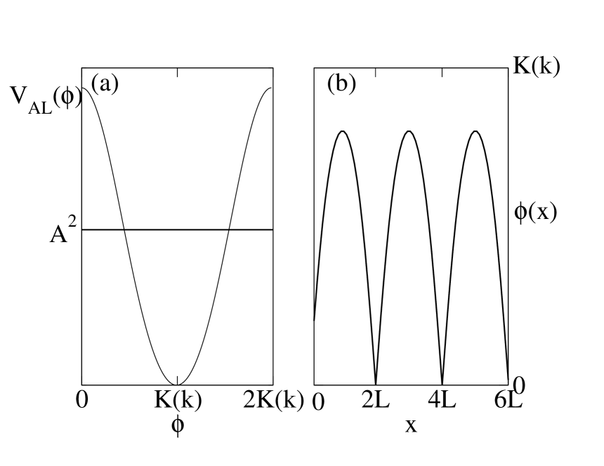
Figure 3: Case II.1 : $0\,\leqslant\,\Gamma\,\leqslant\,k^{\prime}$. (a) The shape of the potential $V_{AL}(\phi)$. The solid horizontal line corresponds to the integration parameter $A^{2}$. (b) The soliton lattice solution [i.e., the field $\phi(x)$] corresponding to the value of $A^{2}$ in (a).

One can compute the energy for one period $2\,L$ of this lattice,

$$E_{SL} = 2\,\sqrt{\displaystyle\frac{2\,|p|}{z_{1}\,-\,z_{2}}}\,\left\{\left[-(z_{1}\,-\,1)\,K(r)\,+\,z_{1}\,\Pi\left(-\,\displaystyle\frac{z_{2}}{z_{1}\,-\,z_{2}},\,r\right)\right]\,\right.$$

$$\left.-\,\Gamma^{2}\,\left[-\,\displaystyle\frac{z_{1}\,-\,1}{1\,-\,z_{1}\,k^{2}}\,K(r)\,+\,\displaystyle\frac{z_{1}\,k^{{}^{\prime}2}}{1\,-\,z_{1}\,k^{2}}\,\Pi\left(-\,\displaystyle\frac{z_{2}\,(1\,-\,z_{1}\,k^{2})}{z_{1}\,-\,z_{2}},\,r\right)\right]\,-\,\displaystyle\frac{a^{2}\,K(r)}{2}\right\}\,.$$

Case II.2 : $k^{\prime}\,<\,\Gamma\,<\,1$

In this case, the potential $V_{AL}(\phi,\,k)$ has two maxima and two degenerate minima in one period $0\,\leqslant\,\phi\,<\,2\,K(k)$. Namely, an absolute maximum, $V_{max}\,=\,|p|\,(1\,-\,\Gamma\,k^{\prime})^{2}$ (for $\phi\,=\,0$); a relative maximum $V^{l}_{max}\,=\,|p|\,(\Gamma\,-\,k^{\prime})^{2}$ [for $\phi\,=\,K(k)$]: and two absolute minima $V_{min}\,=\,0$ situated symmetrically around $K(k)$ [for $\phi\,=\,\mbox{sn}^{-1}\sqrt{(1\,-\,\Gamma\,k^{\prime})/k^{2}},\,2\,K(k)\,-\,\mbox{sn}^{-1}\sqrt{(1\,-\,\Gamma\,k^{\prime})/k^{2}}]$. Note that we used a shift $C\,=\,|p|\,(1\,-\,2\,\Gamma\,k^{\prime}\,+\Gamma^{2})$ in the expression (1) of the potential. A plot of the potential as a function of $\phi$ is given in Fig. 4(a).

The very existence of adjacent degenerate minima of the potential separated by different barriers to the right and to the left (on the $\phi$ axis) implies that in this case one will have two different soliton lattices (and, correspondingly, two different topological single soliton solutions). This is similar to the DSG case leung ; peyrard ; dando .

We follow the same type of integration procedure as that described above.

Case II.2(i) : When $V_{min}\,\leqslant\,A^{2}=|p|\,k^{2}\,a^{2}\,<\,V^{l}_{max}$, i.e., $0\,\leqslant\,a^{2}\,<\,(\Gamma\,-\,k^{\prime})^{2}/k^{2}$, Eq. (6), under the change of variable $z\,=\,\mbox{sn}^{2}(\phi,\,k)$, leads to two different types of solutions.

Solution 1 : for $0\,<\,z\,\leqslant\,z_{2}\,<\,z_{1}\,<\,1$, one has:

$$2\,\sqrt{2\,|p|\,k^{4}}\;x\,=\,\pm\displaystyle\int_{\displaystyle 0}^{\displaystyle z}\displaystyle\frac{d\tilde{z}}{\sqrt{(1\,-\,\tilde{z})\,(z_{1}\,-\,\tilde{z})\,(z_{2}\,-\,\tilde{z})\,(\tilde{z}\,-\,0)}}\,,$$ (22)

where now:

$$z_{1,\,2}\,=\,\displaystyle\frac{2\,(1\,-\,\Gamma\,k^{\prime})\,-\,a^{2}\,k^{2}}{2\,k^{2}}\,\left\{1\,\pm\,\sqrt{1\,-\,\displaystyle\frac{4\,[(1\,-\,\Gamma\,k^{\prime})^{2}\,-\,a^{2}\,k^{2}]}{[2\,(1\,-\,\Gamma\,k^{\prime})\,-\,a^{2}\,k^{2}]^{2}}}\;\right\}\,.$$ (23)

Equation (22) can be integrated using formula 3.147(2) of gradshteyn , thus obtaining:

$$\mbox{sn}^{2}(\phi,\,k)\,=\,\displaystyle\frac{z_{2}\,\mbox{sn}^{2}(w,\,s)}{(1\,-\,z_{2})\,+\,z_{2}\,\mbox{sn}^{2}(w,\,s)}\,,$$ (24)

with $w\,=\,\sqrt{2\,|p|\,k^{4}\,z_{1}\,(1\,-\,z_{2})}\;x$ and the modulus

$$0\,<\,s\,=\,\sqrt{\displaystyle\frac{(1\,-\,z_{1})\,z_{2}}{(1\,-\,z_{2})\,z_{1}}}\,\leqslant\,1\,.$$ (25)

It is a nontopological soliton lattice, with $\phi$ oscillating between $0$ and $\mbox{sn}^{-1}(\sqrt{z_{2}})$ [respectively, $0$ and $-\,\mbox{sn}^{-1}(\sqrt{z_{2}})$]. Its energy for one period $2\,L\,=\,2\,K(s)/\sqrt{2\,|p|\,k^{4}\,z_{1}\,(1\,-\,z_{2})}$ is given by:

$$E_{SL}\,=\,2\,\sqrt{\displaystyle\frac{2\,|p|}{z_{1}\,(1\,-\,z_{2})}}\left\{\left[\displaystyle\frac{(\Gamma\,-\,k^{\prime})^{2}}{k^{2}}\,-\,\displaystyle\frac{a^{2}}{2}\right]\,K(s)\right. + \Pi\left(-\,\displaystyle\frac{z_{2}}{1\,-\,z_{2}},\,s\right)$$ (26)

$$- \left.\Gamma^{2}\,\Pi\left(-\,\displaystyle\frac{z_{2}\,k^{{}^{\prime}2}}{1\,-\,z_{2}},\,s\right)\right\}\,.$$

Solution 2 : for $0\,<\,z_{2}\,<\,z_{1}\,\leqslant\,z\,<\,1$ one obtains from Eq. (6):

$$2\,\sqrt{2\,|p|\,k^{4}}\;x\,=\,\pm\,\displaystyle\int_{\displaystyle z}^{\displaystyle 1}\displaystyle\frac{d\tilde{z}}{\sqrt{(1\,-\,\tilde{z})\,(\tilde{z}\,-\,z_{1})\,(\tilde{z}\,-\,z_{2})\,(\tilde{z}\,-\,0)}}\,,$$ (27)

with $z\,=\,\mbox{sn}^{2}(\phi,\,k)$ and $z_{1,\,2}$ given by Eq. (23). This integral can be solved using formula 3.147(7) of gradshteyn , thus leading to the following nontopological pulse-like lattice

$$\mbox{sn}^{2}(\phi,\,k)\,=\,\displaystyle\frac{z_{1}}{z_{1}\,+\,(1\,-\,z_{1})\,\mbox{sn}^{2}(w,\,s)}\,,$$ (28)

with $w\,=\,\sqrt{2\,|p|\,k^{4}\,z_{1}\,(1\,-\,z_{2})}\;x$ and the modulus $s$ given by the same expression as above, Eq. (25). Of course, one notices immediately that this soliton lattice is different from the previous one, Eq. (24). In one period $2\,L\,=\,2\,K(s)/\sqrt{2\,|p|\,k^{4}\,z_{1}\,(1\,-\,z_{2})}$, $\phi$ oscillates between $\mbox{sn}^{-1}\sqrt{z_{1}}$ and $K(k)$ [respectively, $-\,\mbox{sn}^{-1}\sqrt{z_{1}}$ and $-K(k)$].

The energy corresponding to one period $2\,L$ of this pulse lattice is given by:

$$E_{SL}\,=\,2\,\sqrt{\displaystyle\frac{2\,|p|}{z_{1}\,(1\,-\,z_{2})}}\left\{\left[\displaystyle\frac{(1\,-\,\Gamma\,k^{\prime})^{2}}{k^{2}}\,-\,\displaystyle\frac{a^{2}}{2}\right]\,K(s)\right. + \Pi\left(-\,\displaystyle\frac{1\,-\,z_{1}}{z_{1}},\,s\right)$$ (29)

$$+ \left.\Gamma^{2}\,\Pi\left(-\,\displaystyle\frac{1\,-\,z_{1}}{z_{1}\,k^{{}^{\prime}2}},\,s\right)\right\}\,.$$

A plot of the solutions is given in Fig. 4(b) where the solid and dashed lines correspond, respectively, to the Solution 1 and Solution 2. Therefore, as expected, we obtained two different soliton lattices (with two different limiting cases of topological single solitons). Note that the terms “large” and “small” applied to the topological solitons do not refer, as usual, to the length of the interval they cover in $\phi$ space, but to the height of the barrier they “encounter” peyrard .

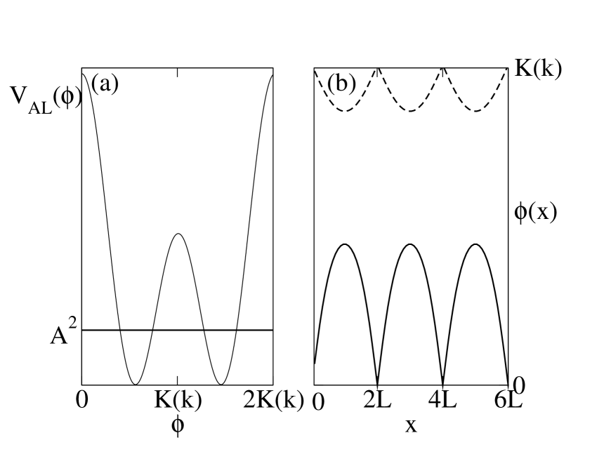
Figure 4: Case II.2 : $k^{\prime}\,<\,\Gamma\,<\,1$. (a) The shape of the potential $V_{AL}(\phi)$. The solid horizontal line corresponds to the integration parameter $A^{2}$. (b) The two nontopological soliton lattice solutions [i.e., the field $\phi(x)$] corresponding to the value of $A^{2}$ in (a); the solid line represents Solution 1 (see the main text), while the dashed line–Solution 2.

Case II.2(ii) : When $V^{l}_{max}\,\leqslant\,A^{2}=|p|\,k^{2}\,a^{2}\,<\,V_{max}$, i.e., $(\Gamma\,-\,k^{\prime})^{2}/k^{2}\,\leqslant\,a^{2}\,<\,(1\,-\,\Gamma\,k^{\prime})^{2}/k^{2}$ there is no soliton lattice solution.

III.3 Case III : $p\,>\,0$ and $q\,\leqslant\,0$

Unlike the last two cases, here $p^{2}$ can be $>$ or $<$ $q^{2}$. However, it turns out that in this case, whatever the value of $\Gamma\,=\,\sqrt{|q|/p}$, the potential $V_{AL}(\phi)$ has only two extrema in one period $0\,\leqslant\,\phi\,<\,2\,K(k)$, namely an absolute minimum $V_{min}\,=\,0$ for $\phi\,=\,0$ and a maximum $V_{max}\,=\,p\,k^{2}\,(1\,+\,\Gamma^{2})$ for $\phi\,=\,K(k)$. Note that we chose $C=p\,k^{2}\,\Gamma^{2}$ in Eq. (1). A plot of the potential $V_{AL}(\phi)$ is given in Fig. 5(a). With $z\,=\,\mbox{sn}^{2}(\phi,\,k)$, Eq. (6) now becomes:

$$2\,\sqrt{2\,p\,k^{4}}\;x\,=\,\pm\,\displaystyle\int_{\displaystyle z}^{\displaystyle 1}\displaystyle\frac{d\tilde{z}}{\sqrt{(z_{1}\,-\,\tilde{z})\,(1\,-\,\tilde{z})\,(\tilde{z}\,-\,z_{2})\,(\tilde{z}\,-\,0)}}\,,$$ (30)

with

$$z_{1,\,2}\,=\,\displaystyle\frac{(1\,+\,\Gamma^{2}\,k^{{}^{\prime}2}\,+\,a^{2}\,k^{2})}{2\,k^{2}}\,\left[1\,\pm\sqrt{1\,-\,\displaystyle\frac{4\,k^{2}\,a^{2}}{(1\,+\,\Gamma^{2}\,k^{{}^{\prime}2}\,+\,a^{2}\,k^{2})^{2}}}\;\right]\,,$$ (31)

$z_{1}\,>\,1\,\geqslant\,z\,>\,z_{2}\,>\,0$. Using the formula 3.147(5) of gradshteyn , one can evaluate the integral in Eq. (30), thus obtaining a nontopological soliton lattice

$$\mbox{sn}^{2}(\phi,\,k)\,=\,\displaystyle\frac{[(z_{1}\,-\,z_{2})\,-\,z_{1}\,(1\,-\,z_{2})\,\mbox{sn}^{2}(y,\,t)]}{[(z_{1}\,-\,z_{2})\,-\,(1\,-\,z_{2})\,\mbox{sn}^{2}(y,\,t)]}\,.$$ (32)

Here $y\,=\,\sqrt{2\,p\,k^{4}\,(z_{1}\,-\,z_{2})}\;x$ and the elliptic modulus:

$$0\,<\,t\,=\,\sqrt{\displaystyle\frac{z_{1}\,(1\,-\,z_{2})}{z_{1}\,-\,z_{2}}}\,\leqslant\,1\,.$$ (33)

In one period $2\,L\,=\,2\,K(t)/\sqrt{2\,p\,k^{4}\,(z_{1}\,-\,z_{2})}$, $\phi$ oscillates between $\mbox{sn}^{-1}\sqrt{z_{2}}$ and $K(k)$ [respectively, $-K(k)$ and $-\,\mbox{sn}^{-1}\sqrt{z_{2}}$]. A plot of the solution is given in Fig. 5(b).

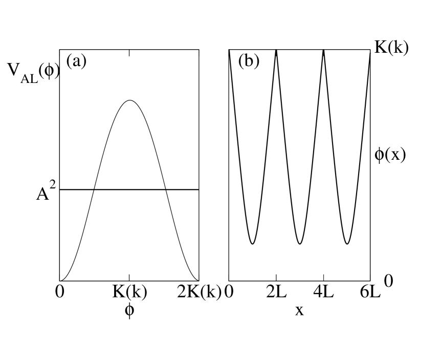
Figure 5: Case III : $p\,>\,0$ and $q\,\leqslant\,0$. (a) The shape of the potential $V_{AL}(\phi)$. The solid horizontal line corresponds to the integration parameter $A^{2}$. (b) The soliton lattice solution [i.e., the field $\phi(x)$] corresponding to the value of $A^{2}$ in (a).

The energy corresponding to one period $2\,L$ of this lattice is:

$$E_{SL} = 2\,\sqrt{\displaystyle\frac{2\,p}{z_{1}\,-\,z_{2}}}\,\left\{\left[z_{1}\,K(t)\,-\,(z_{1}\,-\,1)\,\Pi\left(\displaystyle\frac{1\,-\,z_{2}}{z_{1}\,-\,z_{2}},\,t\right)\right]\,-\,\right.\Gamma^{2}\,k^{{}^{\prime}2}\,\left[\displaystyle\frac{z_{1}}{z_{1}\,k^{2}\,-\,1}K(t)\,-\,\right.$$ (34)

$$\left.\left.-\,\displaystyle\frac{z_{1}\,-\,1}{k^{{}^{\prime}2}\,(z_{1}\,k^{2}\,-\,1)}\,\Pi\left(-\,\displaystyle\frac{(1\,-\,z_{2})\,(z_{1}\,k^{2}\,-\,1)}{k^{{}^{\prime}2}\,(z_{1}\,-\,z_{2})},\,t\right)\right]\,-\,\displaystyle\frac{a^{2}\,K(t)}{2}\right\}\,.$$

IV Single Soliton Solutions of The AL Potential

Having obtained the soliton lattice solutions of the AL problem, it is now straightforward to consider the specific limits of the integration constant $A^{2}$ and to obtain the corresponding single soliton solutions of the Lamé potential and compute their energy.

Cases I.1 and I.2(i) : The limit of a single soliton (that corresponds to the period of the lattice $L\,\rightarrow\,\infty$) is obtained for $t\,\nearrow 1$ [$a^{2}\,\searrow\,0$; $z_{1}\,\rightarrow(1\,-\,\Gamma^{2}\,k^{{}^{\prime}2})/k^{2}$ and $z_{2}\,\searrow\,0$]. One notices that now $\phi$ can vary continuously between $-K(k)$ and $K(k)$ while $x$ explores the whole real axis; therefore, one obtains a topological single-soliton (kink-like) solution,

$${\mbox{sn}(\phi,\,k)}\,=\,\pm\displaystyle\sqrt{\frac{1\,-\,\Gamma^{2}\,k^{{}^{\prime}2}}{1\,-\,\Gamma^{2}\,k^{{}^{\prime}2}+k^{\prime 2}(1-\Gamma^{2}){\mbox{sinh}^{2}(y^{*})}}}\;\,,$$ (35)

where $y^{*}\,=\,\sqrt{2\,p\,k^{2}\,(1\,-\,\Gamma^{2}\,k^{{}^{\prime}2})}\;x$. The corresponding energy of this single kink-like soliton is obtained from Eq. (12), using the relations

$$\mbox{lim}_{r\nearrow 1}\Pi(n^{2},r)=\mbox{lim}_{r\nearrow 1}\frac{K(r)}{1-n^{2}}-\frac{n}{2(1-n^{2})}\,\mbox{ln}\left(\frac{1+n}{1-n}\right)\,.$$ (36)

It may be noted that all the divergences cancel mutually, thus leading to a finite energy of the single soliton:

$$E_{K}\,=\,\sqrt{2\,p\,k^{2}}\left[\displaystyle\frac{1}{k}\,\mbox{ln}\left(\displaystyle\frac{\sqrt{1\,-\,\Gamma^{2}\,k^{{}^{\prime}2}}\,+\,k}{\sqrt{1\,-\,\Gamma^{2}\,k^{{}^{\prime}2}}\,-\,k}\right)\,-\,\Gamma^{2}\,\displaystyle\frac{1}{(\Gamma\,k)}\,\mbox{ln}\left(\displaystyle\frac{\sqrt{1\,-\,\Gamma^{2}\,k^{{}^{\prime}2}}\,+\,(\Gamma\,k)}{\sqrt{1\,-\,\Gamma^{2}\,k^{{}^{\prime}2}}\,-\,(\Gamma\,k)}\right)\right]\,.$$ (37)

Following Manton manton one can compute the asymptotic interaction energy between two solitons in the array, or between a soliton and an anti-soliton. As an illustration we will consider this particular soliton solution; for all the other cases one can follow exactly the same procedure.

From Eq. (35) one obtains the asymptotic shape of the soliton, e.g., for $x\rightarrow+\infty$:

$$\phi_{as}\approx\left[\frac{4(1-\Gamma^{2}\,k^{\prime 2})}{k^{\prime 2}\,(1-\Gamma^{2})}\right]^{1/2}\,\mbox{exp}\left(-\sqrt{2\,p\,k^{2}\,(1-\Gamma^{2}\,k^{\prime 2})}x\right)\,.$$ (38)

Then, if $2\,L\,\gg 1$ is the distance between two solitons in the array, according to manton the asymptotic interaction energy is

$$U(2\,L)\approx-\frac{8\,(2\,p\,k^{2}~{})^{1/2}\,(1-\Gamma^{2}\,k^{\prime 2})^{3/2}}{k^{\prime 2}\,(1-\Gamma^{2})}\,\mbox{exp}\left(-2\,L\,\sqrt{2\,p\,k^{2}\,(1-\Gamma^{2}\,k^{\prime 2})}\right)\,.$$ (39)

If one considers now the small parameter $a^{2}\,\ll\,1$ that measures the distance from the single soliton limit, according to the results in Sec. III we can obtain the asymptotic expression for $2\,L$ as:

$$2\,L\approx\frac{1}{\sqrt{2\,p\,k^{2}\,(1-\Gamma^{2}\,k^{\prime 2})}}\,\mbox{ln}\left(\frac{16\,(1-\Gamma^{2}\,k^{\prime 2})^{2}}{a^{2}\,k^{\prime 2}\,(1-\Gamma^{2})}\right)\,,$$ (40)

and thus

$$U(a^{2})\approx\sqrt{\frac{p\,k^{2}}{2\,(1-\Gamma^{2}\,k^{\prime 2})}}\,a^{2}\,,$$ (41)

that corresponds to a repulsive asymptotic interaction between two solitons in the array. One can consider also the asymptotic interaction energy between a soliton and an anti-soliton and obtains simply $U(a^{2})\approx-\sqrt{\frac{p\,k^{2}}{2\,(1-\Gamma^{2}\,k^{\prime 2})}}\,a^{2}$, i.e., an attractive interaction.

Sine-Gordon Limit

Taking now the limit $k\,\rightarrow\,0$, with $|p|,\,|q|\,\rightarrow\infty$, so that $|p|\,k^{2}\,\rightarrow\,P$ = finite and $|q|\,k^{2}\,\rightarrow\,Q$ = finite, in the expressions of the AL single soliton solution, Eq. (35), one obtains the correct kink-like solution of the sine-Gordon potential in Eq. (2), namely

$$\sin\phi_{sG}\,=\,\pm\mbox{sech}(y^{*})\,,$$ (42)

with $y^{*}\,=\,\sqrt{2\,P\,(1\,-\,\Gamma^{2})}\;x$, and the energy

$$E_{sG}\,=\,2\,\sqrt{2\,P\,(1\,-\,\Gamma^{2})}\,.$$ (43)

Case I.2(ii) : The single soliton limit $L\,\rightarrow\,\infty$ [i.e., $n\,\nearrow\,1$; $a^{2}\,\searrow\,(1\,-\,\Gamma^{2})$, $z_{1}\,\rightarrow 1$, and $z_{2}\,\rightarrow\,(1\,-\,\Gamma^{2})/k^{2}$] reads:

$${\mbox{sn}(\phi,\,k)}\,=\,\pm\,\sqrt{\frac{1-\Gamma^{2}}{1\,-\,\Gamma^{2}+(\Gamma^{2}-k^{\prime 2}){\mbox{sech}^{2}(\omega^{*})}}}\,\;,$$ (44)

with $\omega^{*}\,=\,\sqrt{2\,p\,k^{2}\,(\Gamma^{2}\,-\,k^{{}^{\prime}2})}\;x$. It represents a nontopological soliton, with $\phi$ varying between $K(k)$ and $\mbox{sn}^{-1}(\sqrt{(1\,-\,\Gamma^{2})/k^{2}})$ [respectively, $-\,K(k)$ and $-\,\mbox{sn}^{-1}(\sqrt{(1\,-\,\Gamma^{2})/k^{2}})$] when $x$ runs over the real axis, i.e., it does not connect two adjacent degenerate minima of the potential.

Its energy is obtained from Eq. (16) and reads:

$$E_{S}\,=\,\sqrt{2\,p\,k^{2}}\left[\Gamma^{2}\,\displaystyle\frac{1}{(\Gamma\,k)}\,\mbox{ln}\left(\displaystyle\frac{(\Gamma\,k)\,+\,\sqrt{\Gamma^{2}\,-\,k^{{}^{\prime}2}}}{(\Gamma\,k)\,-\,\sqrt{\Gamma^{2}\,-\,k^{{}^{\prime}2}}}\right)\,-\,\displaystyle\frac{1}{k}\,\mbox{ln}\left(\displaystyle\frac{k\,+\,\sqrt{\Gamma^{2}\,-\,k^{{}^{\prime}2}}}{k\,-\,\sqrt{\Gamma^{2}\,-\,k^{{}^{\prime}2}}}\right)\right].$$ (45)

Case II.1 : Consider now the single soliton limit $r\,\nearrow\,1$ [$a^{2}\,\searrow 0$, $z_{1}\,\rightarrow\,(1\,-\,\Gamma^{2})/k^{2}$, and $z_{2}\,\rightarrow 1$]. One obtains the following topological (i.e., kink-like) soliton:

$${\mbox{sn}(\phi,\,k)}\,=\,\pm\,\sqrt{\displaystyle\frac{1\,-\,\Gamma^{2}}{k^{{}^{\prime}2}\,-\,\Gamma^{2}+(1-\Gamma^{2})\mbox{sinh}^{2}(y^{*})}}\;\mbox{sinh}(y^{*})\,,$$ (46)

with $y^{*}\,=\,\sqrt{2\,|p|\,k^{2}\,(k^{{}^{\prime}2}\,-\,\Gamma^{2})}\;x$, of energy

$$E_{K}\,=\,2\,\sqrt{2\,|p|\,k^{2}}\;\left[\displaystyle\frac{1}{k}\,\mbox{arctan}\left(\displaystyle\frac{k}{\sqrt{k^{{}^{\prime}2}\,-\,\Gamma^{2}}}\right)\,-\,\Gamma^{2}\,\displaystyle\frac{1}{(\Gamma\,k)}\,\mbox{arctan}\left(\displaystyle\frac{(\Gamma\,k)}{\sqrt{k^{{}^{\prime}2}\,-\,\Gamma^{2}}}\right)\right],$$ (47)

where we took the limit $r\,\nearrow\,1$ in Eq. (LABEL:energyII.1) using the relation

$$\mbox{lim}_{r\nearrow 1}\Pi(-n^{2},r)=\mbox{lim}_{r\nearrow 1}\frac{K(r)}{1+n^{2}}+\frac{n}{1+n^{2}}\arctan(n)\,.$$ (48)

Note that one can also consider the limit of the sine-Gordon potential in this case and obtain the correct sine-Gordon soliton.

Case II.2(i) : Solution 1 : Large Topological Kink : Considering the single soliton limit, $s\,\nearrow\,1$ [$a^{2}\,\searrow\,0$, $z_{1,\,2}\,\rightarrow\,(1\,-\,\Gamma\,k^{\prime})/k^{2}$], one obtains a “large” topological kink, that interpolates between two adjacent minima “across” the large barrier $V_{max}$ of the potential:

$${\mbox{sn}(\phi,\,k)}\,=\,\pm\,\sqrt{\displaystyle\frac{1\,-\,\Gamma\,k^{\prime}}{k^{\prime}\,(\Gamma\,-\,k^{\prime})+(1-\Gamma k^{\prime})\mbox{tanh}^{2}(\omega^{*})}}\;\mbox{tanh}(\omega^{*})\,,$$ (49)

with $\omega^{*}\,=\,\sqrt{2\,|p|\,k^{\prime}\,(1\,-\,\Gamma\,k^{\prime})\,(\Gamma\,-\,k^{\prime})}\;x$. Its energy is found from Eqs. (26) and (48) as:

$$E_{K}\,=\,2\,\sqrt{2\,|p|}\,\left[\mbox{arctan}\sqrt{\displaystyle\frac{1\,-\,\Gamma\,k^{\prime}}{k^{\prime}\,(\Gamma\,-\,k^{\prime})}}\,-\,\Gamma\,\mbox{arctan}\sqrt{\displaystyle\frac{k^{\prime}\,(1\,-\,\Gamma\,k^{\prime})}{\Gamma\,-\,k^{\prime}}}\;\right]\,.$$ (50)

Case II.2(i) : Solution 2 : Small Topological Kink : Considering now the single soliton limit $s\,\nearrow\,1$ [$a^{2}\,\rightarrow\,0$, $z_{1,\,2}\,\rightarrow\,(1\,-\,\Gamma\,k^{\prime})/k^{2}$], one obtains a “small” topological kink, that interpolates between two adjacent minima “across” the small barrier $V^{\prime}_{max}$ of the potential:

$${\mbox{sn}(\phi,\,k)}\,=\,\pm\,\sqrt{\displaystyle\frac{1-\Gamma\,k^{\prime}}{1\,-\,\Gamma\,k^{\prime}+k^{\prime}(\Gamma-k^{\prime})\mbox{tanh}^{2}(\omega^{*})}}\,,$$ (51)

with $\omega^{*}\,=\,\sqrt{2\,|p|\,k^{\prime}\,(1\,-\,\Gamma\,k^{\prime})\,(\Gamma\,-\,k^{\prime})}\;x$. Its energy is found from Eqs. (29) and (48):

$$E_{K}\,=\,2\,\sqrt{2\,|p|}\,\left[\Gamma\,\mbox{arctan}\sqrt{\displaystyle\frac{\Gamma\,-\,k^{\prime}}{k^{\prime}\,(1\,-\,\Gamma\,k^{\prime})}}\,-\,\mbox{arctan}\sqrt{\displaystyle\frac{k^{\prime}\,(\Gamma\,-\,k^{\prime})}{1\,-\,\Gamma\,k^{\prime}}}\;\right]\,.$$ (52)

Case III : The single soliton limit $t\,\nearrow\,1$ [$a^{2}\,\searrow\,0$, $z_{1}\,\rightarrow\,(1\,+\,\Gamma^{2}\,k^{{}^{\prime}2})/k^{2}$, and $z_{2}\,\rightarrow\,0$] represents a topological soliton

$${\mbox{sn}(\phi,\,k)}\,=\,\pm\,\sqrt{\displaystyle\frac{(1\,+k^{\prime 2}\,\Gamma^{2})}{1\,+\,\Gamma^{2}\,k^{{}^{\prime}2}+k^{\prime 2}(1+\Gamma^{2})\mbox{sinh}^{2}(y^{*})}}\;,$$ (53)

with $y^{*}\,=\,\sqrt{2\,p\,k^{2}\,(1\,+\,\Gamma^{2}\,k^{{}^{\prime}2})}\;x$. Its energy is given by:

$$E_{K}\,=\,\sqrt{2\,p\,k^{2}}\,\left[\displaystyle\frac{1}{k}\,\mbox{ln}\left(\displaystyle\frac{\sqrt{1\,+\,\Gamma^{2}\,k^{{}^{\prime}2}}\,+\,k}{\sqrt{1\,+\,\Gamma^{2}\,k^{{}^{\prime}2}}\,-\,k}\right)\,+\,2\,\Gamma^{2}\,\displaystyle\frac{1}{(\Gamma\,k)}\,\mbox{arctan}\left(\displaystyle\frac{(\Gamma\,k)}{\sqrt{1\,+\,\Gamma^{2}\,k^{{}^{\prime}2}}}\right)\right]\,.$$ (54)

Here again one can consider the limit of the sine-Gordon potential and obtain the correct sine-Gordon soliton of energy $E_{sG}=2\,\sqrt{2\,P\,(1+\Gamma^{2})}$ .

V Soliton Lattice and Single Soliton Solutions of the Lamé Potential

We shall now demonstrate that having obtained the AL soliton lattice and single soliton solutions, one can immediately obtain the corresponding solutions of the Lamé problem by taking suitable limits of the corresponding AL solutions.

V.1 Lamé Soliton Lattice Solutions

Starting from the AL soliton lattice solutions and considering the limit $\Gamma\rightarrow 0$, we obtain the two following types of Lamé soliton lattice solutions:

Cases I.1 and III ($p>0$) : These lead to type I Lamé soliton lattice solution. The solution is given by Eq. (9) with simpler forms for $z_{1},z_{2}$, namely $z_{1}={1}/{k^{2}}$, $z_{2}=a^{2}$. As a result the Lamé soliton lattice energy has the simpler form

$$E_{SL}=2\,\sqrt{\displaystyle\frac{2\,p}{z_{1}\,-\,z_{2}}}\,\left\{\left[z_{1}\,K(t)\,-\,(z_{1}\,-\,1)\,\Pi\left(\displaystyle\frac{1\,-\,z_{2}}{z_{1}\,-\,z_{2}},\,t\right)\right]\,-\,\displaystyle\frac{a^{2}\,K(t)}{2}\right\}\,.$$ (55)

Case II.1 ($p<0$) : This produces type II Lamé soliton lattice solution. In this case the solution is in fact the same as that given by Eq. (19), except that now $z_{1},z_{2}$ take the simpler values $z_{1}={1}/{k^{2}}$, $z_{2}=1-a^{2}$. As a result the Lamé soliton lattice energy has the simpler form

$$E_{SL}=2\,\sqrt{\displaystyle\frac{2\,|p|}{z_{1}\,-\,z_{2}}}\,\left\{\left[-(z_{1}\,-\,1)\,K(r)\,+\,z_{1}\,\Pi\left(-\,\displaystyle\frac{z_{2}}{z_{1}\,-\,z_{2}},\,r\right)\right]\,-\,\,\displaystyle\frac{a^{2}\,K(r)}{2}\right\}\,.$$ (56)

V.2 Lamé Single Soliton Solutions

We can now easily obtain the corresponding Lamé soliton solutions, either by taking the appropriate limits of the Lamé soliton lattice solutions, or of the AL soliton solutions.

Type I ($p>0$) : For example, considering $\Gamma=0$ in the expressions for the AL soliton solution as given by Eq. (35), the corresponding Lamé one soliton solution turns out to be

$$\mbox{sn}(\phi,\,k)=\frac{1}{\sqrt{1+k^{\prime 2}\,\mbox{sinh}^{2}(y^{*})}}\,,$$ (57)

where $y^{*}=\sqrt{2\,p\,k^{2}}\,x$. The corresponding energy turns out to be

$$E=\sqrt{2\,p}\;\mbox{ln}\left(\frac{1+k}{1-k}\right)\,,$$ (58)

where we have used Eq. (37).

Type II ($p<0$) : Considering $\Gamma=0$ in the expressions for the AL soliton solution as given by Eq. (46) the corresponding Lamé soliton solution turns out to be

$$\mbox{sn}(\phi,\,k)=\frac{\mbox{sinh}(y^{*})}{\sqrt{k^{\prime 2}+\mbox{sinh}^{2}(y^{*})}}\,,$$ (59)

where $y^{*}=\sqrt{2\,|p|\,k^{2}\,k^{\prime 2}}\,x$. The corresponding energy turns out to be

$$E=2\sqrt{2\,|p|}\;\mbox{arctan}\left(\frac{k}{k^{\prime}}\right)\,,$$ (60)

where we have used Eq. (47).

VI Conclusion

We have presented the exact soliton lattice and single soliton solutions, as well as their corresponding energies, for the Associated Lamé equation magnus ; khare ; ganguly in various parameter regimes. In appropriate limits we also obtained the single soliton and soliton lattice solutions of the Lamé equation. The topological and nontopological nature of the different solutions was discussed. As an illustration of Manton’s method manton we also computed, in a particular case, the asymptotic interaction energy between these solitons. In addition to their relevance in the study of nonlinear phenomena, these solutions provide valuable information about domain walls in field theory, materials and many physical systems. It would be worthwhile to analytically study the exact thermodynamical properties of these systems.

VII Acknowledgments

I.B. acknowledges support from the Swiss National Science Foundation. This work was supported in part by the U.S. Department of Energy.

References

- (1) A. Scott, Nonlinear Science (Oxford University Press, New York, 1999); R. Rajaraman, Solitons and Instantons (North-Holland, Amsterdam, 1989).
- (2) K. M. Leung, Phys. Rev. B 26, 226 (1982); Phys. Rev. B 27, 2877 (1983).
- (3) D. K. Campbell, M. Peyrard, and P. Sodano, Physica 19 D, 165 (1986).
- (4) A. Saxena and R. Dandoloff, Phys. Rev. B 58, R563 (1998).
- (5) M. J. Ablowitz, D. J. Kaup, A. C. Newell, and H. Segur, Stud. Appl. Math. 53, 249 (1974); H. P. Mckean, Comm. Pure Appl. Math. 34, 197 (1981).
- (6) S.N. Behera and A. Khare, J. Phys. (Paris) C6, 314 (1981); A. Khare, S. Habib, and A. Saxena, Phys. Rev. Lett. 79, 3797 (1997); S. Habib, A. Khare, and A. Saxena, Physica D 123, 368 (1998).
- (7) F. M. Arscott, Periodic Differential Equations (Pergamon, Oxford, 1981); E. T. Whittaker and G. N. Watson, A Course of Modern Analysis (Cambridge University Press, Cambridge, 1980).
- (8) W. Magnus and S. Winkler, Hill’s Equation (Wiley, New York, 1966).
- (9) A. Khare and U. Sukhatme, J. Math. Phys. 40, 5473 (1999); J. Math. Phys. 42, 5652 (2001).
- (10) A. Ganguly, Mod. Phys. Lett. A 15, 1923 (2000); J. Math. Phys. 43, 1980 (2002).
- (11) N. Gupta and B. Sutherland, Phys. Rev. A 14, 1790 (1976).
- (12) N. S. Manton, Nucl. Phys. B 150, 397 (1979).
- (13) B. Horovitz, Phys. Rev. Lett. 46, 742 (1981).
- (14) L. M. Zhuravchak, Mater. Sci. 36, 33 (2000).
- (15) For the properties of the Jacobi elliptic functions and integrals see I. S. Gradshteyn and I. M. Ryzhik, Tables of Integrals, Series, and Products, (Academic Press, New York, 1980).
- (16) P. F. Byrd and M. D. Friedman, Handbook of Elliptic Integrals for Engineers and Scientists, 2nd Ed. (Springer, Berlin, 1971).