Resonance tongues and patterns in periodically forced reaction-diffusion systems

Abstract

Various resonant and near-resonant patterns form in a light-sensitive Belousov-Zhabotinsky (BZ) reaction in response to a spatially-homogeneous time-periodic perturbation with light. The regions (tongues) in the forcing frequency and forcing amplitude parameter plane where resonant patterns form are identified through analysis of the temporal response of the patterns. Resonant and near-resonant responses are distinguished. The unforced BZ reaction shows both spatially-uniform oscillations and rotating spiral waves, while the forced system shows patterns such as standing-wave labyrinths and rotating spiral waves. The patterns depend on the amplitude and frequency of the perturbation, and also on whether the system responds to the forcing near the uniform oscillation frequency or the spiral wave frequency. Numerical simulations of a forced FitzHugh-Nagumo reaction-diffusion model show both resonant and near-resonant patterns similar to the BZ chemical system.

I Introduction

An oscillator forced by a periodic external perturbation entrains to the forcing for certain values of the perturbation frequency and amplitude. This behavior is observed in a wide range of biological, chemical and physical systems, for example, in circadian rhythms such as the sleep-wake cycle forced by the sun Glass (2001), in the tips of chemical spiral waves forced with light Braune and Engel (1993); Steinbock et al. (1993); Barkely and Mantel (1996); Hakim and Karma (1999); Karma and Zykov (1999), and in arrays of Josephson’s junctions Bohr et al. (1984).

The entrainment to the forcing can take place even when the oscillator is detuned from an exact resonance Arnold (1983); Jensen et al. (1984); Krauskopf (1995). In this case, a periodic force with a frequency $f_{f}$ shifts the oscillator from its natural frequency, $f_{0}$, to a new frequency, $f_{r}$, such that $f_{f}/f_{r}$ is a rational number $m\mbox{:}n$. When the forcing amplitude is too weak this frequency adjustment or locking does not occur; the ratio $f_{f}/f_{r}$ is irrational and the oscillations are quasi-periodic. In dissipative systems frequency locking is the major signature of resonant response. Nearly conservative systems show in addition a large increase in the amplitude of oscillations.

The response of a two-dimensional array of coupled nonlinear oscillators, or of a two-dimensional oscillating field is much less well understood. For a periodically forced single oscillator, the structure in the parameter plane of the forcing frequency $f_{f}$ and amplitude $I$ contains many universal features identified with frequency locking Glazier and Libchaber (1988), but it is unclear if these features persist or change in the more complex case of spatially extended systems where patterns can form. Patterns resulting from time-periodic forcing  Petrov et al. (1997); Lin et al. (2000b, a); Martinez et al. (2002); Yochelis et al. (2002); Dennin (2000); Dolnik et al. (2001a); Gallego et al. (2000, 2001); Goryachev et al. (1998); Hemming and Kapral (2001), spatially periodic forcing Dolnik et al. (2001b), and global feedback Vanag et al. (2000, 2001); Zykov and Engel (2002) have been studied in the past, but a whole phase diagram showing a resonance structure for spatially extended systems has not been reported. Moreover, it is not even clear to what extent the familiar concept of resonance applies to spatially extended systems.

To investigate a phase diagram showing multiple resonances in spatially extended systems, we applied periodic perturbations to a light sensitive form of the Belousov-Zhabotinsky (BZ) chemical reaction-diffusion system and measured the temporal response and pattern formation. In the course of this investigation a new mode of response has been identified. Patterns may fail to lock to the forcing frequency but still respond by showing an $m$-peaked distribution of the oscillation-phase as in resonant patterns. We refer to this response mode as “near-resonant.”

In addition to the nonuniform distribution of the oscillation phase, resonant and near-resonant, patterns can also be characterized by the shape of the phase in the complex phase plane. The phase of unforced spirals has a circular shape in the complex phase plane but forcing breaks the circular symmetry. At high enough forcing this is visible as a $m$-fold symmetry in the phase plane. Examples of $m\mbox{:}1$ patterns observed in the BZ system, where $m\mbox{:}1$=$f_{f}/f_{0}$ and $m=2,3,4$ are shown in Fig 1. Unlike the single oscillator case, a spatially extended system can exhibit phase waves and other phase patterns. In Fig. 1 each pattern is shown in two representations: in the real space $x-y$ plane, and in the complex phase plane.

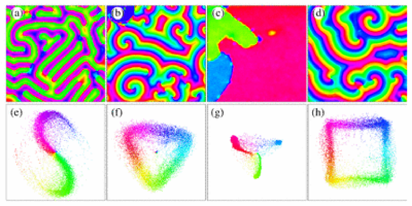
Figure 1: (Color online) Patterns in the periodically forced BZ reaction. (a)-(d) show a $11.5\times 11.5$ $\rm mm^{2}$ size region of patterns formed at different forcing frequencies and amplitudes. The data are processed to show the pattern only near the sub-harmonic response frequency. Patterns (a) and (c) are frequency-locked (resonant). Patterns (b) and (d) are near-resonant but not frequency-locked. The frames (e)-(h) show the same data represented in the complex phase plane, see Lin et al. (2000b). The colors in the phase plane vary with the angle $[0,2\pi]$ and are the key to the pattern images above. See the text for details. (a,e) 2:1 two phase standing-wave pattern; (b,f) 3:1 three phase rotating spiral (c,g) 3:1 three phase standing-wave pattern; (d,h) 4:1 four phase rotating spiral. Chemical conditions are given in BZ (1).

In this paper we construct an experimental phase diagram in the forcing frequency and amplitude parameter plane of resonant and nearly resonant $m\mbox{:}n$ responses and identify the pattern types that lead to the two responses. The experimental set-up and determination of resonance tongues are described in Sec. II and Sec. III, respectively. The qualitatively different patterns observed in the experiments are presented in Sec. IV. A forced reaction-diffusion model, modified FitzHugh-Nagumo equations, is introduced in Sec. V, which is followed by a discussion of the model and the insight it provides into the mechanisms of pattern formation in the experimental system. A general discussion and summary of the results are given in Sec. VI.

II Belousov Zhabotinsky Chemical System

The oscillatory chemical reaction occurs in a thin, porous-glass membrane (0.4 mm thick, 25 mm in diameter), which is in contact on each side with continuously refreshed reservoirs of reagents for the ruthenium-catalyzed Belousov-Zhabotinksy (BZ) reaction dia . Each reservoir is well-stirred and the reagents diffuse from them into the membrane where they react. The chemical concentrations in the reservoirs are given in Ref. BZ (1, 2). Visualization of the patterns is achieved using a low intensity tungsten lamp, which measures the optical density of the concentration patterns in the membrane without affecting the chemical reactions.

For the chemical concentrations used in the present experiments the unforced system exhibits rotating spiral patterns. The patterns are sustained indefinitely in time because the reaction products leave the membrane by diffusion into the reservoirs, and reservoir concentrations are maintained by continuous feeds. We used two different sets of chemical conditions BZ (1, 2), one creating spirals with a higher frequency ($f_{s}=0.072~{}\mbox{Hz}$) and one creating spirals of a lower frequency ($f_{s}=0.020~{}\mbox{Hz}$). Examples of the unforced spiral waves for both sets of chemical conditions are shown in Fig. 2.

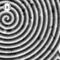
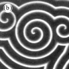
Figure 2: Unforced spiral patterns for the two sets of chemical conditions used for the experiments presented. (a) Spiral waves with a shorter period, $[BrMA]$=0.220 M, $[BrO_{3}^{-}]$=0.230 M BZ (1). (b) Spiral waves with a longer period, $[BrMA]$=0.300 M, $[BrO_{3}^{-}]$=0.136 M BZ (2). The images show a $9$ mm $\times$ $9$ mm region of the pattern. Dark regions correspond to high concentrations of Ru(II). Taken from Martinez et al. (2002). All data reported in this paper are taken under the conditions for the spirals on the left, except for Fig. 4(b).

In addition to the spiral frequency, the BZ system has another natural frequency: the unforced spatially-homogeneous oscillation frequency. Since perturbations always lead ultimately to the formation of spiral waves in the membrane, we determined the homogeneous oscillation frequency $f_{0}$ by the following method. The membrane was exposed to a spatially uniform high-intensity pulse of light for 30 s, which resets the system so the entire membrane is oscillating with the same frequency and phase. The frequency of this spatially uniform oscillation, determined by the chemical kinetics, was found in our previous work to be essentially independent of the chemical concentrations used in our study, $f_{0}=0.020~{}\mbox{Hz}$ Martinez et al. (2002). The uniform oscillations eventually evolve to rotating spiral waves which fill the system. However, the frequency of the spiral waves does depend on the chemical conditions. The ramifications of this dependence will be discussed in the next Section.

III Multiple resonance tongues

The chemical reaction is forced by illuminating it with spatially homogeneous light that is periodically blocked Lin et al. (2000b, a); Martinez et al. (2002); the durations of the illuminated and blocked portions of each cycle are equal, i.e., the intensity modulation is a square wave. To investigate the temporal response of the patterns to the forcing we varied the intensity $I$ and frequency of the periodic light forcing $f_{f}$. The light intensity $I$ is the control parameter for the forcing amplitude. We examined the temporal response to determine which, if any, tongue the pattern belonged to, and examined the existence, shape, and ordering of the resonance tongues (see Sec. III).

III.1 Determining Temporal Resonance

The experimental data were collected as a time-sequence of pattern snapshots. The natural oscillation period of the reaction for the conditions used was about $50$ s. Typically, images were recorded every $2$ s for one hour and a central $240\times 240$ pixel (23 mm $\times$ 23 mm) region of the pattern was analyzed. The Fourier transform of the time series for each pixel was calculated to obtain an average power spectrum for the pattern. Figure 3 shows a typical averaged power spectrum for a resonant pattern when the forcing frequency $f_{f}$ was twice the uniform oscillation frequency $f_{0}$. The largest subharmonic frequency peak appears at $f=f_{f}/2$, as indicated by the vertical line.

Figure 3: Averaged power spectrum for a 2:1 resonant labyrinthine pattern. The response frequency has been normalized to the forcing frequency $f_{f}$. The peak at 0.5 is the subharmonic response to the forcing. The large peak at the forcing frequency ($f=f_{f}$) is due to our imaging method, which captures part of the forcing light output. In this paper we only consider responses subharmonic to the forcing frequency ($f/f_{f}<1)$).

III.2 Tongues

Using the method described in the previous section, we found tongues in the forcing parameter space where the pattern responds at or near $m\mbox{:}n$ resonances. We obtained a phase diagram for each of the two chemical conditions BZ (1, 2), shown in Fig. 4(a),(b). If the peak of the strongest mode subharmonic to the forcing was within $\pm 3\%$ of the forcing frequency, we considered the pattern to be responding to the forcing, and it is included within an $m\mbox{:}n$ resonance region in Fig. 4. This criterion is consistent with the observation of $m$-peaked distributions of the oscillation phase. Some of the patterns meeting this criterion are resonant while others are near-resonant, i.e., they are quasi-periodic patterns with an $m$-peaked phase distribution.

We varied the forcing frequency and intensity in the experiments and explored the temporal resonant response as we moved through the parameter space, and the results are shown in Fig. 4. Each symbol type represents a different $m\mbox{:}n$ resonance. The curves in Fig. 4 are drawn to guide the eye to the tongues in the $f_{f}$-$I$ plane with different $m\mbox{:}n$ responses. Only the largest resonance tongues are plotted. In addition to the $m\mbox{:}1$ tongues (and the 4:3 and 3:2 tongues) shown, we observed several higher order $m\mbox{:}n$ states (e.g., 5:7, 5:1, 6:1, 10:1), which spanned control parameter ranges too narrow to be maintained. In all cases the different $m\mbox{:}n$ tongues were ordered in a Farey sequence, similar to the Devil’s staircase ordering of resonance tongues for two coupled oscillators Bak (1986) and for the homogeneous BZ reaction Maselko and Swinney (1986, 1987).

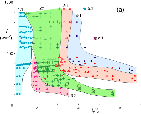
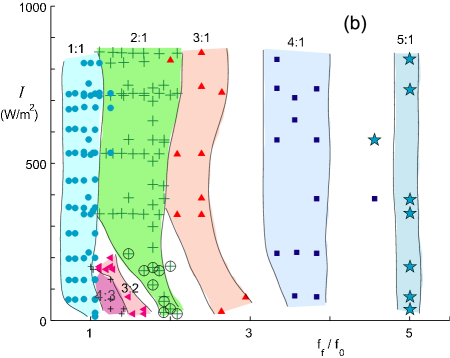
Figure 4: (Color online) The largest $m\mbox{:}n$ tongues observed in the frequency-intensity plane of the spatially extended BZ system. Chemical conditions are those used in Fig. 2(a) BZ (1). (b) The largest $m\mbox{:}n$ tongues observed for the chemical conditions used in Fig. 2(b) BZ (2). The homogeneous frequency in both cases is $f_{0}=0.020$ Hz while the spiral frequency is (a) 0.072 Hz, (b) 0.020 Hz. Each symbol type represents a different $m\mbox{:}n$ response. The patterns (points) within the solid curves respond sub-harmonically with the forcing frequency. The bottom plot is taken from Martinez (2002).

We investigated two different chemical conditions. The chemical conditions that yield 0.072 Hz spirals have $m\mbox{:}n$ tongues that bend toward higher frequency as the light intensity $I$ is decreased [Fig. 4(a)]. For the chemical conditions that yield 0.020 Hz spirals, the tongues do not bend much at low frequency [Fig. 4(b)]. The bending of the tongues is caused by a shifting from $f_{0}$ = 0.02 Hz resonance at high forcing intensity (the uniform oscillation frequency) to the near-resonant response of the spiral wave frequency $f_{s}$ for lower forcing intensity. Since the spiral wave frequency for the data in Fig. 4(b) is the same as the uniform oscillation frequency, the tongues do not bend in that case Martinez et al. (2002); Martinez (2002).

III.3 A quantitative measure of patterns

Spatial Fourier transforms and correlation functions do not capture the temporal aspects of the patterns and did not differentiate the data well because the patterns were often comprised of multiple wavelengths and orientations. Therefore, instead of computing spatial Fourier transforms, we analyzed the temporal Fourier transform calculated for each point in the pattern Lin et al. (2000b, a); Martinez et al. (2002). The power spectrum of the signal, averaged over the spatial pattern, gives information about the strongest frequency response. Additionally, the data were filtered to keep the strongest response and then inverse Fourier transformed. The complex amplitudes of the filtered system give information about the phase distribution of the pattern. Qualitatively different patterns were found to exhibit different shapes in the complex phase-plane representations Lin et al. (2000c) [see Fig. 1(e-h)].

IV Pattern formation

We now describe the asymptotic patterns observed (after the decay of transients) in the $m\mbox{:}1$ tongues for different forcing frequencies and amplitudes. The patterns can be divided into two categories: those which are resonant with the forcing and those which are near-resonant. The resonant patterns are standing waves which lock to the forcing frequency and show $m$ peaks in the phase response. The near-resonant patterns are traveling waves and spiral waves which do not lock to the forcing but still show $m$ peaks in the phase response.

We differentiate the two types of response using their power spectra. If the system is resonant, the response frequency will adjust to be a rational ratio of the forcing frequency. For near-resonant response, however, the frequency does not adjust to be a rational ratio of the forcing frequency. Figure 5 shows the power spectra and corresponding histograms of phase angle for 2:1 near-resonant patterns (spirals) at three forcing frequencies near exact resonance with the spiral wave frequency. The peak of the subharmonic response does not adjust to $f_{f}/2$ (vertical line) as the frequency is varied. The histograms of the phase, however, indicate that there is a two-phase response to the forcing even though there is not exact resonance. In contrast, Fig. 6 shows the power spectra of resonant patterns (standing waves) for three forcing frequencies near exact resonance with the uniform oscillation frequency. In this case the patterns lock to $f_{f}/2$ (shown by the vertical line) even when the forcing is detuned from exact resonance.

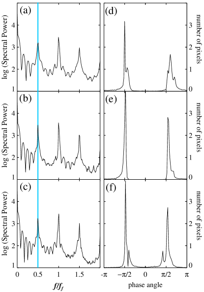
Figure 5: Power spectra and phase histograms for resonant 2:1 standing-wave patterns. Frames (a)-(c) show the power spectra of the response as the forcing frequency is varied across the tongue. The power spectra, normalized to the forcing frequency $f_{f}$, show that the largest response is at exactly half the forcing frequency ($f/f_{f}=0.5$), as indicated by the vertical line. Frames (d)-(f) show histograms of the phase of the pattern near the peak response. The histograms have two peaks corresponding to concentrations of the pattern in regions that are separated in phase by $\pi$. Forcing frequency: (a,d) $f_{f}=0.0333$ Hz, (b,e) $f_{f}=0.0357$ Hz, (c,f) $f_{f}=0.0416$ Hz.

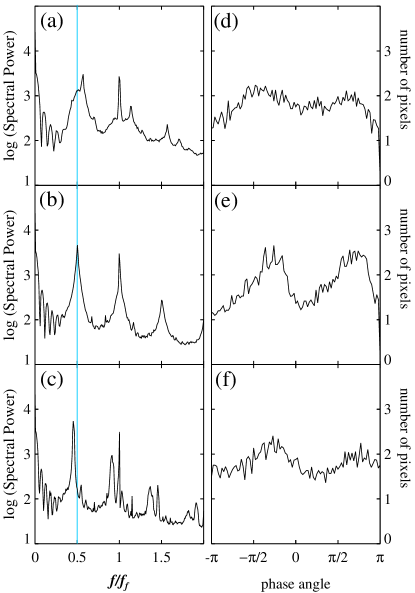
Figure 6: Power spectra and phase histograms for near-resonant 2:1 spiral wave patterns. Frames (a)-(c) show power spectra of the response as the forcing frequency is varied across the tongue. The power spectra, normalized to the forcing frequency $f_{f}$, show that the largest response is nearly half (but not exactly half) the forcing frequency when the forcing is detuned from exact resonance ($f/f_{f}=0.5$ as indicated by the vertical line); thus the spiral wave pattern does not lock to the forcing frequency. The peaks at $f/f_{f}$ = 1 in (a) and (c) include power from the forcing light reflected from the reactor face into the camera. Frames (d)-(f) show histograms of the phase of the pattern near the peak response. The histograms have two peaks which indicates that the pattern is mostly concentrated near one of two phases; the two phases are separated by $\pi$. Forcing frequency: (a,d) $f_{f}=0.0500$ Hz, (b,e) $f_{f}=0.0556$ Hz, (c,f) $f_{f}=0.0625$ Hz.

We now discuss the different types of $m\mbox{:}1$ patterns that we observed.

IV.1 1:1 and 2:1 patterns

In the 1:1 region we observe a resonant response. In this case the entire pattern of chemical concentration oscillates uniformly in space with the forcing frequency, as measured for a range of $f_{f}$ and $I$ values centered at $f_{0}$. The shape of the 1:1 tongue in Fig. 4(a) is different than the shape of the other tongues. The other tongues bend toward higher frequency at low forcing intensities. Instead we find 1:1 uniform patterns at frequencies near $f_{0}$ even at very low forcing intensities We do find spiral patterns at slightly higher frequencies near the bottom of the tongue, but we cannot distinguish 1:1 spiral waves from unforced spiral waves.

Unlike the 1:1 resonant response, for which we observed only a single qualitative pattern, several qualitatively different patterns were observed inside of the 2:1 region. In this region, the oscillation phase responds to either the first or the second forcing cycle, which occurs within a single oscillation cycle of the pattern. The 2:1 patterns are therefore formed from spatial arrangements of regions oscillating at the same frequency but which differ in phase by $\pi$. A description of the different 2:1 patterns observed in the BZ system and in a forced reaction-diffusion model with Brusselator kinetics was given in Lin et al. (2000b).

IV.2 3:1 patterns

In the 3:1 region we observe two qualitatively different types of patterns. At low forcing the 3:1 patterns are rotating spirals, such as those shown in Fig. 7. At low forcing intensity, the spirals have a fairly evenly distributed phase angle and a nearly circular shape in the complex phase plane. At higher forcing intensity, the phase becomes more concentrated in three phases, and the shape in the complex phase plane becomes more triangular. This trend is observable in Fig. 7(b,c).

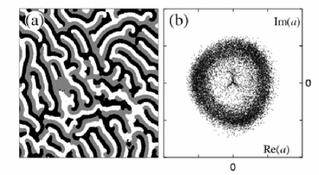
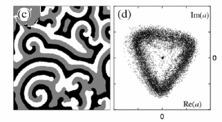
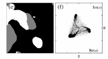
Figure 7: Patterns observed in the 3:1 resonance region for different forcing amplitudes (the patterns are shown after filtering). The response is shown in the $x-y$ plane (left) and complex phase plane (right). (a,b) Spiral waves in the bottom of the 3:1 region, $I=269\rm{W/m}^{2}$, $f_{f}=0.1251$ Hz. (c,d) Spiral waves in the middle of the 3:1 region, $I=382\rm{W/m}^{2}$, $f_{f}=0.0667$ Hz. (d,e) Standing wave patterns found at the top of the 3:1 region, $I=863\rm{W/m}^{2}$, $f_{f}=0.0769$ Hz.

An abrupt transition from traveling wave patterns to what appear to be standing wave patterns is observed in the 3:1 resonance region as the forcing amplitude was increased. The transition between these pattern types was observed at a fixed forcing frequency of 0.075 Hz as $I$ was increased past roughly 460 W/m², and was also observed for fixed forcing amplitudes in a range of 300 to 400 W/m² when $f_{f}$ was increased past roughly 0.065 Hz. The experimental resolution is not enough to determine the functional form of the transition.

The 3:1 standing wave patterns with stationary or nearly stationary fronts consist of irregularly shaped domains differing in phase by $2\pi/3$ (see Fig. 7). Often the fronts are rough, i.e., have short wavelength modulations that appear stable over a hundred oscillation cycles of the pattern, as can be seen in the standing wave pattern pictured in Fig. 1(c).

The fronts in the standing-wave patterns are either stationary or propagate on a time scale orders of magnitude larger than the unforced spiral period. If the latter is the case, the patterns are not precisely standing waves, and over a longer time could evolve to other patterns such as large and slowly rotating three-phase spiral waves. If so, these patterns could be understood to be observations of the 3:1 patterns predicted by the forced complex Ginzburg-Landau (CGL) equation Gallego et al. (2001); Coullet and Emilsson (1992).

IV.3 Other patterns

Rotating four-phase spiral patterns, e.g. Fig. 1(d,h), are the only pattern type observed in the 4:1 resonance region of the BZ experiments. A detailed description of 4:1 resonance in the forced CGL equation and in the FitzHugh-Nagumo and Brusselator reaction-diffusion models was given in Lin et al. (2000c). In those models a bifurcation from four-phase traveling patterns to two-phase 4:1 resonant standing-wave patterns was found Lin et al. (2000a). This bifurcation has not been observed in our experiments, perhaps because the forcing light intensity $I$ available may be insufficient to reach the bifurcation. Another possibility is that the patterns observed were at a frequency near four times the spiral wave frequency $f_{s}$ instead of near four times the uniform oscillation frequency $f_{0}$. In the experimentally accessible range of $I$, we have observed only 4:1 spiral wave patterns and none of the more complicated pattern behavior found in the 4:1 forced CGL model Hemming (2003).

Patterns such as the 2:1 Bloch fronts and spiral waves discussed in Coullet et al. (1990); Coullet and Emilsson (1992); Elphick et al. (1997) and the 4:1 rotating spirals discussed in Lin et al. (2000a) are not resonant since they are all traveling patterns.

Finally, we present examples of near resonant 5:1 and 6:1 patterns in Fig. 8 and Fig. 9, respectively.

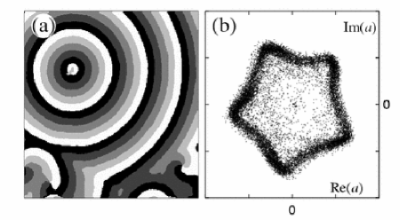
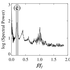
Figure 8: BZ spirals observed in the 5:1 resonance region at $I$ = 661 W/m², $f_{f}$ = 0.100 Hz. The patterns are filtered to keep only the frequencies shown by the gray band in (c). (a) Phase patterns in $x-y$ plane. (b) Phase in complex plane. (c) Average temporal power spectrum. (d) Histogram of phase angle.

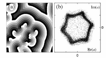
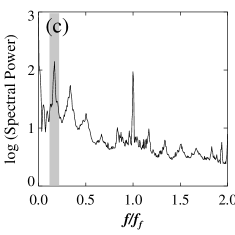
Figure 9: BZ spirals observed in the 6:1 resonance region at $I$ = 475 W/m², $f_{f}$ = 0.1001 Hz. The patterns are filtered to keep only the frequencies shown by the gray band in (c). (a) Phase patterns in the $x-y$ plane. (b) Phase in complex plane. (c) Average temporal power spectrum. (d) Histogram of phase angle.

V Reaction-diffusion model

As a model for a periodically forced oscillatory system we use a version of the FitzHugh-Nagumo (FHN) reaction-diffusion equations

$$u_{t} = u-u^{3}-v+\nabla^{2}u\,,$$ (1a)

$$v_{t} = \epsilon\left[u-\left(a_{1}+\gamma\sin\omega_{f}t\right)v\right]+\delta\nabla^{2}v\,,$$ (1b)

where the fields $u(x,y)$ and $v(x,y)$ represent concentrations of chemicals in a simple model of a chemical system. We add explicit time dependence to the FHN system as parametric sinusoidal forcing with amplitude $\gamma$ and frequency $\omega_{f}$. The parameter $\epsilon$ is the ratio of the time scales of $u$ and $v$ and $\delta$ is the ratio of the diffusion rates of $u$ and $v$. In the following we fix the parameters $\epsilon=0.1$, $\delta=0.1$, $a_{1}=0.5$, and vary the forcing frequency and amplitude.

In the absence of forcing, $\gamma=0$, the equations have a spatially uniform solution $u=v=0$. The parameter $\epsilon$ controls the stability of this solution. When $\epsilon>2$, $u=v=0$ is stable, and at $\epsilon=2$, there is a Hopf bifurcation to uniform oscillations. Beyond the Hopf bifurcation Eqs. (1) also support traveling phase waves. Our numerical investigations are conducted in the parameter range where uniform oscillations and phase waves both exist. In two space dimensions phase waves typically form into rotating spirals, each one organized around a core where the amplitude of oscillations is zero. For the parameters above, the spiral wave frequency ($\omega_{s}\approx 0.237$) is faster than the homogeneous oscillation frequency ($\omega_{s}\approx 0.215$); once formed, spiral waves spread to fill the entire system.

V.1 Periodic forcing and data analysis

A sinusoidal parametric forcing, homogeneous in space, is applied by choosing a nonzero $\gamma$ parameter in Eq. (1). As in the BZ experiment, when the forcing amplitude is high enough the system can lock at rational ratios of the forcing frequency. Frequency locking of spatially uniform solutions to Eq. (1) occurs in tongue-shaped regions in the $\omega_{f}-\gamma$ parameter plane. A complete diagram of the pattern-forming tongues was not computed for the FHN equation with this forcing scheme. We have only investigated certain resonances to compare with the BZ chemical experiment. Our numerical investigations show that the size and shape of different $m\mbox{:}n$ tongues depends on the exact form of the parametric forcing in Eqs. (1) Bold and Hagberg (2003). Tongue diagrams obtained by forcing other terms of the FHN model were presented in studies of locking to uniform oscillations in the oscillatory FHN model Kharrazian (2000); Sailer (2001?). A diagram for the 2:1 tongue of a periodically forced Brusselator reaction-diffusion system was given in Ref. Lin et al. (2000b).

The data from the numerical solutions of the forced FHN equation are processed to extract phase information, as in the experimental system. Every 1.4 time units, we store the values of $u(x,y)$ and $v(x,y)$ at each computational grid point $x_{i},y_{j}$. The discrete Fourier transform is applied to the time variable of $u(x,y,t)$ to get the frequency response $\hat{u}(x,y,\omega)$ for each point in the pattern. The averaged power spectrum of the signal,

$$P(\omega)=\frac{1}{N_{x}N_{y}}\sum_{i,j}|{\hat{u}(x_{i},x_{j})}|^{2}\,,$$ (2)

where $N_{x}$ and $N_{y}$ are the number of grid points in the $x$ and $y$ directions, is then examined to determine the system response. The response frequency is isolated from the signal $\hat{u}$ using a box filter centered at the response frequency, $\omega_{r}$ with width $\Delta$. The filtered signal is then inverse Fourier transformed, which gives the response in time, $a(x,y,t)$.

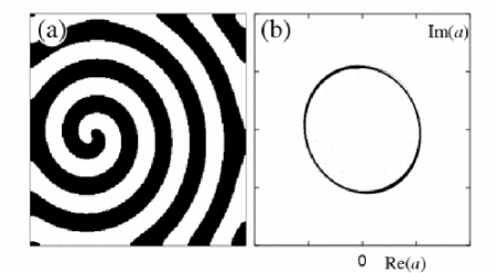
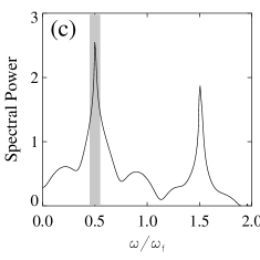
Figure 10: Spiral wave in Eq. (1) with periodic forcing at nearly twice the spiral wave frequency. The patterns are filtered to keep only the frequencies shown by the gray band in (c). (a) Phase pattern in $x-y$ plane. (b) Phase in complex plane. (c) Average temporal power spectrum. (d) Histogram of phase angle. Parameters: $\gamma=0.5,\omega_{f}=0.474$, $x=[0,256]$, $y=[0,256]$.

Figure 10 shows an example of a 2:1 spiral wave with the peak frequency response at $\omega_{f}/2$ displayed clearly in the power spectra. The filtered signal $a$ in $x-y$ domain is shown in Fig. 10(a), and Fig. 10(b) shows the same data plotted in the complex phase plane. The width of the filter is shown in the power spectrum by the gray band (see Fig. 10(c)). The phase plane shows that different parts of the spatial domain are in different relative phases, all oscillating at the same frequency. The phase is not uniformly distributed but has peaks near two phases that become apparent in the histogram of the phase angle shown in Fig. 10(d).

V.2 Pattern Formation

The FHN equations (1) have two intrinsic frequencies, the uniform oscillation frequency, $\omega_{0}$, and the spiral wave frequency $\omega_{s}$. For some choices of parameters (e.g. $\delta=1$) these two frequencies are the same, but for the parameters chosen in this study the two frequencies differ ($\omega_{s}>\omega_{0}$). Because of this there are two possible different resonant response conditions: when the forcing is a rational multiple of either $\omega_{0}$ or $\omega_{s}$. In the following we will show how the FHN equations (1) respond to forcing in both of those cases. In the BZ experiment this distinction is harder to make.

V.3 Patterns at $m\mbox{:}n$ response of the uniform oscillation frequency

When the forcing is a rational multiple of the uniform oscillation frequency $\omega_{0}$, spatially uniform solutions of Eq. (1) are found for a range of forcing frequency $\omega_{f}$ and amplitude $\gamma$. The $m\mbox{:}n$ frequency-locked solutions form tongue shaped regions in the $\omega_{f}-\gamma$ parameter plane (Arnol’d tongues). The shape of the resonant tongues depends on the exact form of the forcing Bold and Hagberg (2003).

As in the BZ experiment, patterns may form in the frequency-locked tongues. Resonant pattern solutions consist of standing waves connecting regions of different phases. For example, in the 2:1 resonance, standing waves consist of fronts between regions in space that are oscillating at the same frequency but out of phase by $\pi$. The fronts must be stationary for the pattern to be strictly frequency locked, since any motion indicates that the phase is drifting and thus, at least in the vicinity of a front, the frequency is also slowly changing.

A 2:1 resonance is found when the forcing frequency is nearly twice the uniform oscillation frequency, $\omega_{f}\sim 2\omega_{0}$. For sufficiently high forcing amplitude, the system frequency locks at $\omega_{f}/2$, in one of two phases separated by $\pi$. Patterns form from the two phases. At low forcing amplitude the pattern is a two phase rotating spiral wave and thus is near-resonant but not strictly frequency-locked since the spiral rotates slowly (relative to the forcing period). At higher forcing amplitude the pattern is standing waves. The spiral waves and standing waves are similar to those found in the BZ experiment and in forced complex Ginzburg-Landau and Brusselator models Petrov et al. (1997); Bertram (1999); Lin et al. (2000b); Yochelis et al. (2002).

In the 3:1 resonance the system responds at one-third the forcing frequency, $\omega_{r}=\omega_{f}/3$, and the patterns consist of spatial regions of three locked phases. In our exploration in forced FHN model we find that the three locked phases organize into rotating spiral waves.

Patterns in a forced 4:1 FHN model consist of four-phase spiral waves and two-phase standing waves and are discussed in detail in Ref. Lin et al. (2000a).

The domain in parameter space where frequency locked patterns (standing waves) exist is different from that of frequency locked uniform solutions. Recently it was discovered that frequency locked standing wave patterns can exist outside of the resonant tongue of spatially uniform solutions or that spatial instabilities can reduce the range of resonant patterns Yochelis et al. (2003a, b).

V.4 Patterns at $m\mbox{:}n$ response of the spiral wave frequency

When the forcing frequency is close to a rational multiple of the spiral wave frequency, the spiral does not frequency lock to the forcing but still shows a near-resonant response. This can be seen in the nonuniform phase distribution of the forced spiral waves, with $m$ peaks for waves forced near an $m\mbox{:}n$ resonance. For example, forcing the spiral wave at approximately twice the spiral frequency, $\omega_{f}\approx 2\omega_{s}$, causes the spiral to respond by shifting the relative oscillation phases within the spiral to be concentrated near two phases, as shown in Figures 12(d)-(f).

Figure 12 shows the spiral wave response when the forcing frequency is scanned through the spiral frequency. The maximum response in the power spectrum is not $\omega_{f}/2$ when the forcing frequency is not exactly twice the spiral wave frequency; the pattern is not frequency locked but it is near-resonant. In contrast to a quasi-periodic response farther away from resonance Lin et al. (2000b), near-resonant patterns exhibit a nonuniform distribution in the histograms of the phase angle. This distribution is farthest from uniform when the forcing is closest to $\omega_{f}/2$, see Fig. 12(d)-(f).

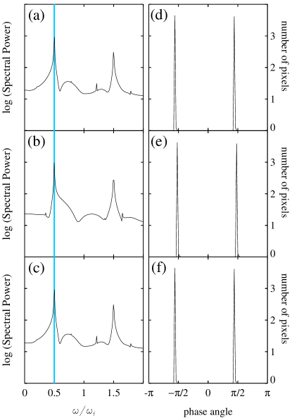
Figure 11: Resonant standing-wave response in the 2:1 forced FHN Eq. (1). (a)-(c) Power spectra for three different forcing frequencies near $2\omega_{0}$. The frequencies are normalized to the forcing frequency $\omega_{f}$. The peak subharmonic response is exactly at half the forcing frequency, even when the forcing is not exactly $2\omega_{0}$, as indicated by the vertical line at $\omega/\omega_{f}=0.5$. (d)-(e) Histograms of the distribution of phase angle for the spiral waves in (a)-(c). The two peaks in the distribution show that the pattern response is primarily in two phases separated by an angle of $\pi$. Parameters: $\gamma=3.0$, (a) $\omega_{f}=0.349$, (b) $\omega_{f}=0.370$, (c) $\omega_{f}=0.419$.

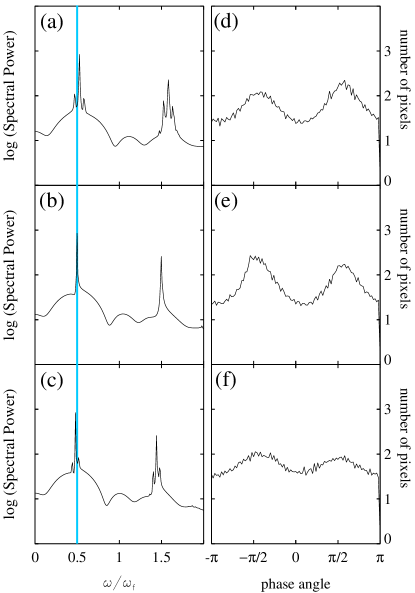
Figure 12: Response of a 2:1 forced spiral wave in the FHN Eq. (1). (a)-(c) Power spectra for three different forcing frequencies (a) $\omega_{f}/2<\omega_{s}$, (b) $\omega_{f}/2\approx\omega_{s}$, (c) $\omega_{f}/2>\omega_{s}$. The solid line indicates $\omega_{f}/2$. When the forcing is not exactly in resonance the peak response in the power spectra differs from $\omega_{f}/2$ indicating that the spiral is not frequency locked. (d)-(e) Histograms of the distribution of phase angle for the spiral waves in (a)-(c). The two peaks in the distribution show that the spiral wave responds to the forcing by redistributing the internal relative distribution of the phase even though the pattern is not frequency locked. Parameters: $\gamma=0.3$, (a) $\omega_{f}=0.465$, (b) $\omega_{f}=0.474$, (c) $\omega_{f}=0.493$.

Forcing near other resonances of the spiral wave frequency also results in a near-resonant response, with the number of peaks in the phase histogram corresponding to the $m\mbox{:}n$ resonance. In the 3:1 resonance we observe three peaks and in the 4:1 resonance we find four peaks. Other spiral resonances such as 5:1 and 6:1 can also be found. These results are similar to observations near-resonant spirals in the of the BZ experiment.

To characterize the effect of the forcing on the spiral wave pattern, we measured the deviation of the phase from a uniform distribution. For an unforced spiral wave, the histogram of the phase near the spiral frequency is flat, indicating that the phase is uniformly distributed between $-\pi$ and $\pi$. When the spiral wave is nearly 2:1 resonant, the histogram shows two peaks that are separated by $\pi$ in the phase distribution. Figures 12(d)-(f) show.

The nonuniform phase response was measured by the chi-square statistic relative to the uniform distribution. The phase data at $k=256\times 256$ computational grid points was binned into 100 equal size bins between $-\pi$ and $\pi$. The chi-square statistic is

$$\chi^{2}=\sum_{i}\frac{(N_{i}-E)^{2}}{E}\,,$$ (3)

where $N_{i}$ is the value in bin $i$ and $E=k/100$ is the expected value. Figure 13 shows the dependence of $\chi^{2}$ on the forcing amplitude $\gamma$ when the forcing frequency is near $2\omega_{s}$. The $\chi^{2}$ value increases exponentially as the forcing amplitude is increased from near zero. The nonzero value of $\chi^{2}$ at $\gamma=0$ is due to small fluctuations in the phase of our finite size sample.

Figure 13: The $\chi^{2}$ statistic of the deviation in the phase distribution of the 2:1 forced spiral wave from a uniform (unforced spiral) distribution. The $\chi^{2}$ value increases exponentially as the forcing amplitude increases. Parameters in Eq. 1: $\epsilon=0.1,\delta=0.1,a_{1}=0.5,\omega_{f}=0.465$.

VI Discussion

The BZ chemical system in an open gel-reactor was used to identify multiple tongues, each with a different $m\mbox{:}n$ resonance, in the forcing frequency-amplitude parameter plane. Such a phase diagram has not been previously reported for a spatially extended oscillatory system. The resonance tongues are found to be ordered in a Farey sequence, similar to the Devil’s staircase ordering of resonance tongues for two coupled oscillators Bak (1986) and for the homogeneous BZ reaction Maselko and Swinney (1986, 1987).

The diffusively coupled oscillations we measure respond to external forcing either resonantly or at near resonance (quasi-periodically but with an $m$-peaked phase distribution). The resonant patterns are standing waves that frequency lock to a $m\mbox{:}n$ ratio of the forcing frequency. In this case, a power spectrum of the resulting resonant pattern shows a single primary peak at $f_{f}/m$, along with its higher harmonics, and the phase distribution has $m$ peaks shifted by $2\pi/m$. The near-resonant patterns are traveling waves which do not lock to a ratio of the forcing frequency but have a response near $f_{f}/m$. However, the phase distribution still shows $m$ peaks. This near-resonant quasi-periodic behavior is different from quasi-periodicity farther away from resonance, where patterns have a flat phase distribution Lin et al. (2000b); Bertram (1999).

Both the resonant and near-resonant behavior are also observed in a FitzHugh-Nagumo reaction-diffusion model with sinusoidal periodic forcing, similar to the experiments.