Spectral properties and classical decays in quantum open systems

Abstract

We study the relationship between the spectral properties of diffusive open quantum maps and the classical spectrum of Ruelle-Pollicott resonances. The leading resonances determine the asymptotic time regime for several quantities of interest - the linear entropy, the Loschmidt echo and the correlations of the initial state. A numerical method that allow an efficient calculation of the leading spectrum is developed using a truncated basis adapted to the dynamics.

I Introduction

The study of the emergence of classical features in systems ruled by quantum mechanics is as old as quantum mechanics itself. When the quantum system is isolated and the evolution unitary, these features appear in the WKB semiclassical limit, which is of paramount importance in establishing the quantum classical correspondence in integrable systems. In its more modern form, the EBK quantization rule EBK , it shows the direct connection between tori in phase space and quantized eigenfunctions in Hilbert space. In chaotic systems, the relationship is more subtle and is embodied in the celebrated Gutzwiller trace formula Gutzwiller , relating sets of unstable periodic orbits to the density of states. The limits of applicability of these semiclassical methods and the insight they provide on the quantum dynamics of isolated chaotic systems has inspired most of the recent research in the area of quantum chaos.

In open quantum systems, on the contrary, the emergence of classical features has been studied mainly in the time evolution of a different set of observables, most notably the rate of linear entropy growth (or purity decay)zurek , the Loschmidt echo or fidelity peres ; losch ; prosen and the decay of correlations Srednicki . These studies have demonstrated that in certain well defined regimes for chaotic systems the classical Lyapunov exponent governs these rates and that the evolution of localized quantum densities in phase space becomes classical.

In this article we consider this question from the point of view of the spectral properties of the classical and quantum propagators. Classical densities evolve according to the Liouville equation whose solution can be written in terms of a propagator called Perron-Frobenius operator(PF)PF . It is unitary on $\mathbb{L}^{2}$. However, for chaotic systems, correlation functions exhibit oscillations and exponential decay. The decay rates are given by the poles of the resolvent of the PF operator, the so-called Ruelle-Pollicott (RP) resonancesruel . By limiting the resolution of the functional space, one can effectively truncate the PF to a nonunitary operator of finite size (say $N\times N$) with a spectrum lying entirely inside the unit circle, except for the simply degenerate eigenvalue 1. In the, properly taken, limit of infinite size and no coarse graining, the isolated eigenvalues turn out to be the RP resonancesblank ; nonn . As shown in garma , the linear entropy and the Loschmidt echo, for asymptotic times much longer than the Ehrenfest time, also show characteristic decay rates governed by the classical RP resonancesruel . Experimental evidence of this dependence on RP resonances was observed for the first time in sridhar . Our approach is similar in spirit to the calculations performed on the sphere for the dissipative kicked top by Haake and collaborators haak ; webe ; braun , Fishman susy ; khod and, for the baker’s map, by Hasegawa and Saphir hase . We model the unitary dynamics by means of a quantum map and implement a diffusive superoperator represented by a Kraus sum. Two recent works by Blank, et al. blank and Nonnenmachernonn provide a rigorous theoretical underpinning to our calculations for quantum and classical maps on the torus.

The plan of the paper is as follows. Section II provides a short account of the quantization procedure for maps acting on a classical surface with periodic boundary conditions in both coordinates and momenta, i.e. a torus. In Sec.III we implement the open system dynamics with the definition of a diffusion superoperator represented as a Kraus sum. The general spectral properties of both the unitary and the noisy part, as well as those of the combined action are studied. Sec.IV deals with the relationship between the classical and the quantum resonances and, utilizing recently proved theorems blank ; nonn , how they coincide in specific ranges of $\hbar$ and of the noise strength. As a consequence we show that the asymptotic time behaviour of several quantities is classical and depends on the Ruelle-Pollicott resonaces closer to the unit circle. A numerical method that allows the calculation of the leading spectrum of resonances is developed. Sec.V illustrates this correspondence taking the perturbed Arnold cat map as an example. We relegate to the Appendix some notation concerning the spectral decomposition of superoperators and the details of the numerical method.

II Unitary dynamics on the torus $\mathbb{T}^{2}$

We picture the classical phase space as a square of unit area with sides identified. The classical transformations will map this square onto itself, thus providing a simple model of Hamiltonian area preserving dynamics. The fact that the phase space has finite area brings some well known special features to the quantization that we briefly review. Refs. ozorivas ; Miquel provide a more extensive account.

II.1 The Hilbert space

As the phase space has finite area, which we normalize to unity, the Hilbert space ${\cal H}_{N}$ is finite and its dimension $N$ sets the value of Planck’s constant to $\hbar=(2\pi N)^{-1}$. The position and momentum bases are then sets of discrete states $|\,q\,\rangle,|\,p\,\rangle,~{}q,p=0,..N-1$ which are related by the discrete Fourier transform (DFT) of dimension $N$

$$\langle\,p|\,q\,\rangle={1\over\sqrt{N}}\,\text{e}^{-{2\pi{\rm i}\over N}pq}.$$ (1)

A vector $|\,\varphi(t)\,\rangle$ in ${\cal H}_{N}$ characterizes pure states of the system and can be represented by the amplitudes $\langle q|\varphi\rangle,\langle p|\varphi\rangle$ in the coordinate or momentum basis, respectively.

In the description of open systems it is imperative to represent states by a density operator $\hat{\rho}$. They form a subset of self-adjoint, positive semidefinite matrices with unit trace in ${\cal H}_{N^{2}}\stackrel{{\scriptstyle\mbox{\footnotesize def}}}{{=}}{\cal H}_{N}\otimes{\cal H}_{N}^{*}$ , the space of complex $N\times N$ matrices, usually called in this context Liouville space. While Hilbert space is the natural arena for unitary dynamics, this much larger Liouville space sets the stage for the more general description of open quantum dynamics. It acquires the structure of a Hilbert space with the usual introduction of the matrix scalar product

$$(\hat{A},\hat{B})=\mbox{Tr}(\hat{A}^{\dagger}\hat{B}).$$ (2)

where $\hat{A},\hat{B}\in{\cal H}_{N^{2}}$. Linear transformations in this space are termed superoperators, they map operators into operators and are represented by $N^{2}\times N^{2}$ matrices. In Appendix A we review the various notations and properties related to this space.

II.2 Translations on the torus

The usual translation operator in the infinite plane $\mathbb{R}^{2}$ is

$$\hat{T}_{(q,p)} = \text{e}^{-{i\over\hbar}(q\hat{P}-p\hat{Q})}$$

$$= \text{e}^{-{i\over\hbar}q\hat{P}}\text{e}^{{i\over\hbar}p\hat{Q}}\text{e}^{{i\over 2\hbar}qp}$$

$$= \hat{U}^{q}\hat{V}^{p}\text{e}^{{i\over 2\hbar}qp},$$ (4)

where $\hat{U}$ and $\hat{V}$ generate shifts in the position and momentum eigenbasis respectively. On the torus the main difference is that the infinitesimal translation operators $\hat{P},\hat{Q}$ with the usual commutation rules cannot be defined because position and momentum eigenstates are discrete. However, finite translation operators $\hat{U}$ and $\hat{V}$ that have the property

$$\hat{V}^{p}\hat{U}^{q}=\hat{U}^{q}\hat{V}^{p}\text{e}^{i{2\pi\over N}qp}$$ (5)

can be defined and they generate finite cyclic shifts in the respective bases schwinger . The $N\times N$ grid of coordinate and momentum states constitutes the quantum phase space for the torus. Eq. (5) allows a definition of a translation operator $\hat{T}_{(q,p)}:{\cal H}_{N}\to{\cal H}_{N}$, $q,p$ integers, analog to Eq. (II.2). The action of $\hat{T}$ on position and momentum eigenstates is

$$\hat{T}_{(q_{1},p_{1})}|\,q\,\rangle = \exp\left[i{2\pi\over N}p\left(q+{q_{1}\over 2}\right)\right]|\,q+q_{1}\,\rangle$$ (6)

$$\hat{T}_{(q_{1},p_{1})}|\,p\,\rangle = \exp\left[-i{2\pi\over N}q\left(p+{p_{1}\over 2}\right)\right]|\,p+p_{1}\,\rangle.$$ (7)

These equations confirm that $\hat{T}_{(q_{1},p_{1})}$ are indeed phase space translations. They satisfy the Weyl group composition rule

$$\hat{T}_{(q_{1},p_{1})}\hat{T}_{(q_{2},p_{2})}=\hat{T}_{(q_{1}+q_{2},p_{1}+p_{2})}\text{e}^{i{\pi\over N}(p_{1}q_{2}-q_{1}p_{2})}.$$ (8)

The $N^{2}$ translations $\hat{T}_{(q,p)},p,q=0,..N-1$ satisfy the orthogonality relation

$$\mbox{Tr}(\hat{T}^{\dagger}_{(q,p)}\hat{T}_{(q^{\prime},p^{\prime})})=N\delta_{qp,q^{\prime}p^{\prime}}$$ (9)

thus constituting an orthogonal basis for the Liouville space ${\cal H}_{N^{2}}$.

The expansion of any operator $\hat{A}$ in this basis constitutes the chord ozorivas or characteristic function representation. This representation assigns to every $\hat{A}\in{\cal H}_{N^{2}}$ the c-number function $a(q,p)=N^{-1}\,\mbox{Tr}(\hat{A}\hat{T}_{(q,p)}^{{}^{\dagger}})$ and therefore every operator has the expansion

$$\hat{A}=\sum_{q,p}a(q,p)\hat{T}_{(q,p)}.$$ (10)

For representation purposes we also use a basis of “phase point ” operators that constitute the Weyl, or center ozorivas , representation. In this basis the density operator is the discrete Wigner function of the quantum state. The peculiar features of the discrete Wigner function for Hilbert spaces of finite dimension have been described recently in Miquel .

II.3 Unitary Dynamics: quantum maps

A classical map is a dynamical system that usually, but not exclusively, arises form the discretization of a continuous time system (by means of a Poincaré section, for example). Although it is always possible, by integration of the equations of motion, to derive the map from a Hamiltonian, this connection is rather involved and in many instances it is more useful to model specific features of Hamiltonian dynamics by directly specifying the map equations without going through the integration step. The same is true in quantum mechanics: instead of modeling the Hamiltonian operator and integrating it to obtain the unitary propagator, it is simpler to model directly the unitary map. Classically an area preserving map is characterized by a finite canonical transformation and the corresponding quantum map is the unitary propagator that represents this canonical transformation. There are no exact and systematic procedures to realize this correspondence. On the 2-dimensional plane $\mathbb{R}^{2}$ relatively standard procedures (see OdAbook ) give an approximation of the propagator in the semiclassical limit as

$$U(q_{1},q_{2})=\left({i\over\hbar}{\partial^{2}S\over\partial q_{1}\partial q_{2}}\right)^{1/2}\exp\left[{i\over\hbar}S(q_{2},q_{1})\right],$$ (11)

where $S$ is the action along the unique classical path from $q_{1}$ to $q_{2}$, and where for simplicity we do not consider the existence of multiple branches and Maslov indices. Only for linear symplectic maps on $\mathbb{R}^{2}$ this unitary propagator is exact, and then $S$ is minus the quadratic generating function of the linear transformation. On the other hand, several ad-hoc procedures for the quantization of specific maps have been devised: some integrable (translationsschwinger and shears) and chaotic maps, such as cat maps hannay ; OdA , baker maps balazs ; saraceno and the standard map izra . Also all maps of a “kicked” nature, realized as compositions of non-commuting nonlinear shears can be quantized, as well as periodic time dependent Hamiltonians BerryVoros . Once the quantum propagator has been constructed, the advantages of using quantum maps to model specific features of quantum dynamics become apparent. The propagator $\hat{U}$ is a unitary $N\times N$ matrix, propagation of a pure state is achieved simply by matrix multiplication, and finally the classical limit is obtained by letting $N\to\infty$.

In Liouville space the evolution of the density operator $\hat{\rho}$ by the map $\hat{U}$ is given by

$$\hat{\rho}^{\prime}=\hat{U}\rho\hat{U}^{\dagger}.$$ (12)

As a linear map acting on ${\cal H}_{N^{2}}$ Eq. (12) can be written as

$$\hat{\rho}^{\prime}=\hat{U}\otimes\hat{U}^{\dagger}(\hat{\rho})=\text{{{U}}}(\hat{\rho}),$$ (13)

In what follows the notation $\hat{U}\otimes\hat{U}^{\dagger}$ is meant to be equivalent to the $Ad(U)$ notation customary in group theory. The linear operator $\text{{{U}}}\stackrel{{\scriptstyle\mbox{{\footnotesize def}}}}{{=}}\hat{U}\otimes\hat{U}^{\dagger}$ is a unitary $N^{2}\times N^{2}$ matrix.

III Noisy Dynamics

Realistic quantum processes always involve a certain degree of interaction between system and environment. In this case the evolution of the system is not unitary and requires a description in Liouville space. This loss of unitarity leads to decoherence and to the emergence of classical features zurekRMP03 ; pazLH in the evolution. When the environment is taken into account the evolution of the system is governed by a master equation, which takes the form of a hierarchy of integro-differential equations. A drastic simplification follows from the assumption that the environment reacts to the system sufficiently fast, in such a manner that the system looses all prior memory of its state, i.e. that the evolution is Markovian. . The resulting Lindblad equation L ; Perc

$$\frac{{\rm d}\hat{\rho}}{{\rm d}t} = -{{\rm i}\over\hbar}[\hat{H},\hat{\rho}]+$$ (14)

$$\mbox{\hskip 7.11317pt}+{1\over\hbar}\sum_{j}(\hat{L}_{j}\hat{\rho}\,\hat{L}_{j}^{\dagger}-\frac{1}{2}\hat{L}_{j}^{\dagger}\hat{L}_{j}\hat{\rho}-\frac{1}{2}\hat{\rho}\,\hat{L}_{j}^{\dagger}\hat{L}_{j}).$$

determines the evolution of open quantum systems through a Hamiltonian $\hat{H}$ that governs the unitary noiseless evolution and the Lindblad $\hat{L}_{i}$ operators that model the interaction with the environment. The particular structure of the equation ensures that the evolution preserves the total probability, the positive semi-definiteness and hermiticity of the density matrix. The infinitesimal propagator is a linear operator in Liouville space which can be integrated to yield a finite linear mapping

$$\hat{\rho}=\text{{{S}}}(\hat{\rho}_{0}).$$ (15)

This mapping, as a reflection of the structure of the Lindblad equation, also has a particular form that guarantees the preservation of the general properties of the density operator. The general form, called the Kraus representation Kraus is

$$\text{{{S}}}(\hat{\rho})=\sum_{\mu}\hat{M}_{\mu}\hat{\rho}\hat{M}^{\dagger}_{\mu}=\Bigg{[}\sum_{\mu}\hat{M}_{\mu}\otimes\hat{M}^{\dagger}_{\mu}\Bigg{]}(\hat{\rho}).$$ (16)

The only further restriction on the $\hat{M}_{\mu}$ operators arises from the preservation of the trace that requires

$$\sum_{\mu}\hat{M}_{\mu}^{\dagger}\hat{M}_{\mu}=\hat{I}.$$ (17)

In what follows we will select them from a certain complete family, with a specific norm. In that case the representation takes a more general form

$$\text{{{S}}}(\hat{\rho})=\sum_{\mu}c_{\mu}\hat{M}_{\mu}\hat{\rho}\hat{M}^{\dagger}_{\mu}$$ (18)

where now the positivity requirements are $c_{\mu}\geq 0$ and

$$\sum_{\mu}c_{\mu}\hat{M}_{\mu}^{\dagger}\hat{M}_{\mu}=\hat{I}.$$ (19)

Within this general framework, just as in the case of quantum maps, we have the choice of modeling the noise through the Lindblad operators or directly in terms of the integrated form via the Kraus operators. In what follows we choose the latter and thus we model the evolution by specifying a quantum map to represent the unitary evolution followed by a noisy step, modeled by its Kraus superoperator form. An evolution of the density matrix specified in this way is known in the literature preskill ; chuang ; schumacher ; caves as a quantum operation. It includes the special case of unitary evolution when the sum is limited to only one term. In that case, and only then, the dynamics is reversible. A general superoperator has no inverse.

III.1 Quantum coarse grained dynamics

We are interested in modeling the effect of a small amount of noise on the evolution of an otherwise unitary quantum map bian ; nonn ; braun ; garma . We assume that the one step propagator results from the composition of two superoperators. The first is the unitary propagator U and the second is a quantum diffusion superoperator $\text{{{D}}}_{\epsilon}$, defined by

$$\text{{{D}}}_{\epsilon}=\sum_{q,p}c_{\epsilon}(q,p)\hat{T}_{(q,p)}\otimes\hat{T}_{(q,p)}^{{}^{\dagger}},$$ (20)

that introduces decoherence. The linear form of the full propagator is

$$\text{{{L}}}_{\epsilon}=\text{{{D}}}_{\epsilon}\circ\text{{{U}}}$$ (21)

and its action on a density matrix $\hat{\rho}$ is

$$\text{{{L}}}_{\epsilon}(\hat{\rho})=\sum_{q,p}c_{\epsilon}(q,p)\hat{T}_{(q,p)}\hat{U}\hat{\rho}\hat{U}^{\dagger}\hat{T}_{(q,p)}^{{}^{\dagger}}.$$ (22)

As the Kraus operators in this case are unitary the condition (19) becomes simply

$$\sum_{q,p}c_{\epsilon}(q,p)=1.$$ (23)

Subject to this condition $c_{\epsilon}(q,p)$ can be an arbitrary positive function of $q$ and $p$. Its significance in terms of coarse graining is clear: as long as $c_{\epsilon}(q,p)$ is peaked around $(0,0)$ and of width $\epsilon$, the action that follows the unitary step consists in displacing the state incoherently over a phase space region of order $\epsilon$. To avoid a net drift in any particular direction, $c_{\epsilon}(q,p)$ must be an even function of the arguments $q$ and $p$. From this imposition and the fact that

$$\hat{T}_{(q,p)}^{{}^{\dagger}}=\hat{T}_{(-q,-p)}$$ (24)

it follows, from the properties of the matrix scalar product (2) that $\text{{{D}}}_{\epsilon}$ is hermitian (see App. A for details on the scalar product).

The spectral properties of the separate superoperators U and $\text{{{D}}}_{\epsilon}$ are simple to obtain. If the Floquet spectrum of the quantum map is

$$\hat{U}|\,\phi_{k}\,\rangle={\rm e}^{{\rm i}\xi_{k}}|\,\phi_{k}\,\rangle$$ (25)

then the spectrum of U is unitary and given by

$$\text{{{U}}}(|\,\phi_{k}\,\rangle\langle\,\phi_{j}|)={\rm e}^{{\rm i}(\xi_{k}-\xi_{j})}|\,\phi_{k}\,\rangle\langle\,\phi_{j}|.$$ (26)

To obtain the spectrum of $\text{{{D}}}_{\epsilon}$ we use the composition rule (8) to show that

$$\hat{T}_{(q,p)}\hat{T}_{(\mu,\nu)}\hat{T}_{(q,p)}^{\dagger}=\exp\left[{\rm i}\frac{2\pi}{N}(\nu q-\mu p)\right]\hat{T}_{(\mu,\nu)}.$$ (27)

We then derive

$$\text{{{D}}}_{\epsilon}\left(\hat{T}_{(\mu,\nu)}\right) = \sum_{q,p}c_{\epsilon}(q,p)\hat{T}_{(q,p)}\hat{T}_{(\mu,\nu)}\hat{T}_{(q,p)}^{{}^{\dagger}}$$ (28)

$$= \sum_{q,p}c_{\epsilon}(q,p)\exp\left[{\rm i}{2\pi\over N}(\nu q-\mu p)\right]\hat{T}_{(\mu,\nu)}$$

$$= \widetilde{c_{\epsilon}}(\mu,\nu)\hat{T}_{(\mu,\nu)}.$$

Therefore, the $N^{2}$ eigenvalues of $\text{{{D}}}_{\epsilon}$ are given by the $2D$ discrete Fourier transform $\widetilde{c_{\epsilon}}(\mu,\nu)$ of the coefficients $c_{\epsilon}(q,p)$. The eigenfunctions are the translation operators themselves. Hence, using the bra-ket notation described in appendix A, the spectral decomposition of $\text{{{D}}}_{\epsilon}$ is

$$\text{{{D}}}_{\epsilon}=\sum_{\mu,\nu}\Big{|}T_{(\mu,\nu)}\Big{)}\widetilde{c_{\epsilon}}(\mu,\nu)\Big{(}T_{(\mu,\nu)}\Big{|},$$ (29)

in analogy with Eq. (76).

Physically, the action of $\text{{{D}}}_{\epsilon}$ is quite simple in the chord representation (10): if $\hat{\rho}$ is expanded as

$$\hat{\rho}=\sum_{\mu,\nu}\rho_{\mu,\nu}\hat{T}_{(\mu,\nu)}$$ (30)

then

$$\text{{{D}}}_{\epsilon}(\hat{\rho})=\sum_{\mu,\nu}\widetilde{c_{\epsilon}}(\mu,\nu)\rho_{\mu,\nu}\hat{T}_{(\mu,\nu)}.$$ (31)

Thus the coefficients in the chord representation are suppressed selectively according to $\widetilde{c_{\epsilon}}(\mu,\nu)$.

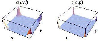
Figure 1: The left pane $\widetilde{c_{\epsilon}}(\mu,\nu)$ shows the eigenvalues of $\text{{{D}}}_{\epsilon}$ for $\epsilon=0.15$ and $N=100$. The DFT of this function generates the coefficients $c_{\epsilon}(q,p)$ (right pane) of the Kraus representation of $\text{{{D}}}_{\epsilon}$ of Eq. (20).

It is evident from Eqs. (20) and (29) that the diffusion superoperator thus defined can be specified indistinctly either by $c_{\epsilon}(q,p)$ or by $\widetilde{c_{\epsilon}}(\mu,\nu)$ . For an efficient numerical implementation of its action we have found convenient to specify the latter as

$$\widetilde{c_{\epsilon}}(\mu,\nu)=\text{e}^{-{1\over 2}\left({\epsilon N\over\pi}\right)^{2}\left(\sin^{2}[\pi\mu/N]+\sin^{2}[\pi\nu/N]\right)},$$ (32)

This is a smooth Gaussian-like periodic function of the integer variables $\mu$ and $\nu$. For large values of $N$ it is very close to the Gaussian

$$\widetilde{c}(\mu,\nu)\simeq\text{e}^{-\epsilon^{2}(\mu^{2}+\nu^{2})/2}$$ (33)

This means that the action of $\text{{{D}}}_{\epsilon}$ will leave essentially unaltered the coefficients $\rho_{\mu,\nu}$ in a region of size $\sim 1/(\epsilon N)$ (Fig. 1, left) around the origin while strongly suppressing those outside. The backward DFT of $\widetilde{c_{\epsilon}}(\mu,\nu)$ does not have a simple analytic expression but from general properties of the DFT it will also be a Gaussian like function with the complementary width $\sim\epsilon/2\pi$ (Fig. 1,right).

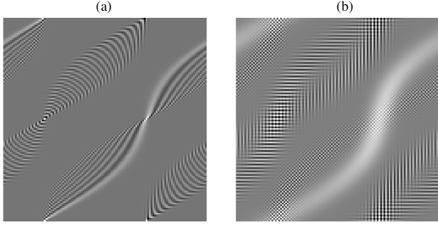
Figure 2: Display of the action of $\text{{{D}}}_{\epsilon}$. Panel (a) shows the Wigner function after the step U has been applied to a position state ($\rho_{0}=|\,q_{0}\,\rangle\langle\,q_{0}\,|$). Panel (b) shows the state after the full propagator $\text{{{L}}}_{\epsilon}=\text{{{D}}}_{\epsilon}\circ\text{{{U}}}$ has acted. The map is the perturbed cat map of Eq. (64)$k=0.02$, $N=60$, $\epsilon=0.25$.

The action of $\text{{{D}}}_{\epsilon}$ progressively washes out the quantum interference. This fact is clearly seen if the density matrix is represented by the Wigner function. On the torus the Wigner function exhibits two different types of interference. The stretching and folding produce quantum interference between different parts of the extended state. Additionally, the periodicity of the torus introduces interference between the state and its images. In Fig. 2 we show the difference between the unitary and the noisy evolution of a coordinate state by a nonlinear map. The two types of interference are clearly seen. The long wavelength fringes on the convex side are produced by nonlinearities. The short wavelength fringes correspond to the images. The effect of the noise can be seen on (Fig. 2(b)) : the classical part of the state (in white) has been broadened and the long wavelength interference has been significantly erased. This process continues at each step of the propagation and the quantum state becomes more and more mixed and more and more classical.

III.2 Spectrum of the quantum coarse gained propagator

In this section we study the general features of the spectrum of the combined action of the unitary map and the coarse graining operator, given by (Eq. (22)). For finite values of $\epsilon$ and $N$, $\text{{{L}}}_{\epsilon}$ is a convex sum of unitary matrices and is therefore a completely positive, contracting superoperator. Its spectrum has the following properties:

• It is unital i.e. it has a trivial non-degenerate unit eigenvalue corresponding to the uniform density $\hat{\rho}_{\infty}=\hat{I}/N$.

• The remaining spectrum is entirely contained inside the unit circle and symmetric with respect to the real axis. The pair of complex conjugate eigenvalues correspond to hermitian conjugate eigenoperators.

• As $\sqrt{(\text{{{L}}}_{\epsilon}\circ\text{{{L}}}_{\epsilon}^{\dagger})}=\text{{{D}}}_{\epsilon}$ the eigenvalues of $\text{{{D}}}_{\epsilon}$ are also the singular values of $\text{{{L}}}_{\epsilon}$. Therefore the spectrum is contained exactly in the annulus

  $$\text{e}^{-\left({\epsilon N\over\pi}\right)^{2}}\leq|\lambda_{i}|\leq\text{e}^{-\frac{1}{2}\left(\epsilon N\over\pi\right)^{2}\left(\sin^{2}[\pi/N]\right)}$$ (34)

  In the limit of large $N$ we can thus write

  $$-\left(\frac{N\epsilon}{\pi}\right)^{2}\leq\ln|\lambda_{i}|\leq-\frac{\epsilon^{2}}{2}.$$ (35)

  The singular values accumulate near the origin, thus forcing most of the eigenvalues of $\text{{{L}}}_{\epsilon}$ to be near zero. On the other hand the allowed eigenvalue region extends exponentially close to the unit circle in the limit $\epsilon\to 0$.

• The superoperator is not normal, and therefore has distinct left and right eigenoperators corresponding to each eigenvalue. The left and right eigenvalue problems are then posed as follows for each pair of complex conjugate eigenvalues $\lambda,\lambda^{*}$

  $$\text{{{L}}}_{\epsilon}\hat{R}_{i}=\lambda_{i}\hat{R}_{i} \text{{{L}}}_{\epsilon}\hat{R}_{i}^{\dagger}=\lambda_{i}^{*}\hat{R}_{i}^{{\dagger}}$$ (36)

  $$\text{{{L}}}_{\epsilon}^{\dagger}\hat{L}_{i}=\lambda_{i}^{*}\hat{L}_{i} \text{{{L}}}_{\epsilon}^{\dagger}\hat{L}_{i}^{\dagger}=\lambda_{i}\hat{L}_{i}^{\dagger}$$ (37)

  where $\hat{L}_{i},\,\hat{R}_{i}$ conform a biorthogonal set

  $$\mbox{Tr}\left(L_{i}^{\dagger}R_{j}\right)=\mbox{Tr}\Big{(}L_{i}R_{j}\Big{)}=\mbox{Tr}\left(L_{i}^{\dagger}R_{j}^{\dagger}\right)=\delta_{i,j}.$$ (38)

  and we assume the normalization $\mbox{Tr}\left(L_{i}^{\dagger}L_{i}\right)=\mbox{Tr}\left(R_{i}^{\dagger}R_{i}\right)=1$ In particular, corresponding to $\lambda_{0}=1$ we choose $\hat{L}_{0}=\hat{R}_{0}=\hat{I}/N$ and therefore all the remaining eigenoperators are traceless.

• The spectral decomposition of $\text{{{L}}}_{\epsilon}$ then becomes

  $$\text{{{L}}}_{\epsilon}=\sum_{i}|\,R_{i}\,)\lambda_{i}(\,L_{i}|.$$ (39)

The exact numerical calculation of the spectrum is hampered by the need to diagonalize very large non-hermitian matrices of dimension $N^{2}\times N^{2}$ for values of $N$ large enough to extract semiclassical features from the spectrum. In Section IV.2 we develop a method, specially adapted to chaotic systems, that takes account of the dynamics of the map to extract the part of the leading spectrum relevant to asymptotic time behavior.

IV Quantum classical correspondence

Chaotic evolution in phase space implies exponential stretching and squeezing of initially localized densities. On a timescale of the order of the Ehrenfest time $t_{\hbar}$, significant quantum corrections to the classical evolution inevitably appear. However, essentially classical features emerge from quantum chaotic dynamics when decoherence is introduced, even in the limit of no decoherence. In this section we relate the spectra of the propagators of densities (both classical and quantum) with the underlying, mainly asymptotic, behavior of time dependent quantities.

Consider the classical analog for the propagation of densities in phase space. If $f(\mathbf{x})$ is a classical map, and $\mathbf{x}=(q,p)$ a point in phase space, then the evolution of a probability density is governed by

$$\rho^{\prime}(\mathbf{y})=\int\delta(\mathbf{y}-f(\mathbf{x}))\rho(\mathbf{x})\mbox{d}\mathbf{x}=\left[{\cal L}\rho\right](\mathbf{y})$$ (40)

where $\mathbf{y}=(q^{\prime},p^{\prime})$ and ${\cal L}$ is the Perron-Frobenius (PF) operatorPF . It is unitary on the space of square integrable functions $\mathbb{L}^{2}$, and infinite dimensional. However, one is mostly interested in the decay properties of observables much smoother than $\mathbb{L}^{2}$. When the functional space on which ${\cal L}$ operates is restricted by smoothness, the spectrum of PF changes drastically, moving to the inside of the unit circle. This smoothing can be attained by convolution with a self adjoint compact (on $\mathbb{L}^{2}$) coarse graining operator ${\cal D}_{\epsilon}$ nonn ; cgsup , where $\epsilon$ is the coarse graining parameter. The coarse grained PF takes the form

$${\cal L}_{\epsilon}={\cal D}_{\epsilon}\circ{\cal L},$$ (41)

(notice the analogy with Eq. (21)). ${\cal D}_{\epsilon}$ damps high frequency modes in $\mathbb{L}^{2}$ and thus effectively truncates ${\cal L}$ to a nonunitary operator. There is substantial difference, however, between the spectrum of the PF for a regular map and for a chaotic map. As the coarse graining $\epsilon$ tends to zero, parts of the spectrum of ${\cal L}_{\epsilon}$ for a regular map can be arbitrarily close to the unit circle. On the contrary, for a chaotic map there is a finite gap for any value of $\epsilon>0$. The isolated eigenvalues which remain inside the unit circle as $\epsilon\to 0$ are the Ruelle-Pollicot resonances. Rughrugh and more recently Blank, et al. blank made formal descriptions of the spectrum of PF for Anosov maps on the torus using tailor-made Banach spaces adapted to the dynamics. Moreover Blank, et al. use this to analyze resonances of noisy propagators and prove that these resonances are stable, i.e. independent of $\epsilon$ in the limit of small coarse-graining . Blum and Agamagam proposed a numerical method to approximate the classical spectrum using similar concepts.

A formal and very thorough recent work by Nonnenmachernonn explores the characteristics of propagators, both classical and quantum, with noise for maps on the torus, both regular and chaotic. In that work its is proved that, in the limit $N\to\infty$, the spectrum of the coarse grained quantum propagator $\text{{{L}}}_{\epsilon}$, for fixed $\epsilon$, tends to that of the coarse grained PF ${\cal L}_{\epsilon}$(nonn Theorem 1). These two theorems, taken together, provide a solid framework for the numerical calculation of quantum resonances of torus maps and of their classical manifestations.

IV.1 Asymptotic behavior

The time evolution the von Neumann entropy was used by Zurek and Pazzurek to characterize quantum chaotic systems. They conjectured that the rate of increase of the von Neumann entropy of the decohering (chaotic) system is independent of the strength of the coupling to the environment and is ruled by the Lyapunov exponents. Thus classicality emerges naturally and correspondence even for chaotic systems is recovered when decoherence is considered. This assertion was extensively tested numerically monte ; bian ; garma ; patta mainly for the linear entropy (closely related to the purity) which is a lower bound of the von Neumann entropy. Other quantities, like the Loschmidt echolosch which also display a noise independent Lyapunov decay. have also become of interest recently, especially in the context of quantum information processing and computing. Besides the linear entropy, in this section we study the asymptotic behavior of the autocorrelation function and the Loschmidt echo.

For purely chaotic systems, after the initial spread governed by the Lyapunov exponent, a state $\hat{\rho}$ evolved $n$ times approaches asymptotically $\hat{\rho}_{\infty}=\hat{I}/N$ and all time dependent quantities saturate to a constant value. The rate at which these quantities saturate is given by the largest eigenvalue, in modulus, smaller than one. Since, according to nonn the spectrum of $\text{{{L}}}_{\epsilon}$ approaches that of ${\cal L}_{\epsilon}$, then the universality of these decays can also be used to characterize quantum chaos.

To display the decay towards $\hat{\rho}_{\infty}$ we subtract it from the initial state. Thus given an arbitrary state $\hat{\rho}$, we define

$$\hat{\rho}_{0}=\hat{\rho}-{\hat{I}\over N},$$ (42)

were it is clear that $\mbox{Tr}(\hat{\rho}_{0})=0$. Thus in all computations instead of evolving an initial state, we evolve an initial traceless pseudo-state such as the one defined in Eq. (42), orthogonal to $\hat{\rho}_{\infty}$. Thus, we study how the distance between the initial state and the equilibrium state evolves. For example, for the linear entropy, after the initial Lyapunov behavior, which ends at about the Ehrenfest time ($n_{E}\sim\ln N$), instead of saturation to the equilibrium state $\rho_{\infty}$, we expect to get an unbound growth which represents how this distance decreases exponentialy, and the exponent is proportional to $|\lambda_{1}|$.

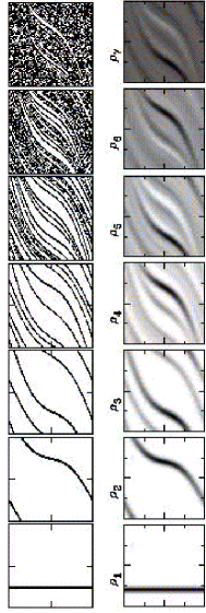
Figure 3: Quantum-classical correspondence for the noisy propagator. The top row shows repeated applications of the Perron-Frobenius operator of the perturbed Arnold cat of Eq. (64), to an initial classical (position) state. The bottom row shows the Husimi representation of $\rho_{0},\ldots,\rho_{6}$, where $\rho_{0}$ is a position eigenstate ($N=150$, $\epsilon=0.2$, $k=0.02$).

Assuming for simplicity that all the eigenvalues are nondegenerate, and that $\hat{R}_{i}$, $i=0,\ldots,N^{2}-1$, are the right eigenfunctions (see App. A) then the expansion of $\hat{\rho}_{0}$ in terms of $\hat{R}_{i}$ is

$$\hat{\rho}_{0}=\sum_{i\neq 0}r_{i}\hat{R}_{i},$$ (43)

were $r_{i}=\mbox{Tr}(\hat{L}_{i}^{\dagger}\hat{\rho}_{0})$ and $\hat{L}_{i}$ is the left eigenfunction. The pseudo state $\hat{\rho}_{0}$ evolved $n$ times, is given by

$$\hat{\rho}_{n}=\text{{{L}}}_{\epsilon}^{n}\hat{\rho}_{0}=\sum_{i\neq 0}r_{i}\lambda_{i}^{n}\hat{R}_{i}.$$ (44)

If the eigenvalues are ordered decreasingly, according to $1>|\lambda_{1}|\geq|\lambda_{2}|\geq\ldots\geq\lambda_{N^{2}-1}$, then $\hat{\rho}_{0}$ is a sum of exponentially decaying modes. Suppose that $\lambda_{1}$ is real, then it is clear from Eq. (44) that

$$\hat{\rho}_{n}\to r_{1}\lambda_{1}^{n}\hat{R}_{1}$$ (45)

as $\ n\to\infty$. Hence the asymptotic decay to the uniform density is ruled by $\lambda_{1}$. As a consequence any quantity which depends explicitly on $\hat{\rho}_{n}$ shows an exponential decay. Such is the case for the autocorrelation function

$$C(n)=\mbox{Tr}(\hat{\rho}_{0}^{\dagger}\hat{\rho}_{n})$$ (46)

From Eq. (45) we get, for large $n$,

$$C(n)\to|r_{1}|^{2}\lambda_{1}^{n}+\ldots$$ (47)

where we used the fact that $\mbox{Tr}(\hat{R}_{1}^{\dagger}\hat{R}_{1})=1$. If $\lambda_{1}$ is complex then

$$\hat{\rho}\sim\lambda_{1}^{n}r_{1}\hat{R}_{1}+\lambda_{1}^{*^{n}}r_{1}^{*}\hat{R}_{1},$$

and C(n) oscillates around $\lambda_{1}^{n}$ (oscillation also appears if, for example, $|\lambda_{2}|\approx|\lambda_{1}|$). Similarly, we can see that the linear entropy

$$S_{n}=-\ln\left[\mbox{Tr}(\hat{\rho}^{2}_{n})\right]$$ (48)

grows linearly with $2n$. Once again, using Eq. (45), the linear entropy for large $n$ is

$$S_{n} \sim -\ln\left[|r_{1}|^{2}|\lambda_{1}|^{2n}\mbox{Tr}\left(\hat{R}_{1}^{\dagger}\hat{R}_{1}\right)\right]$$ (49)

$$= -2n\ln\left[|\lambda_{1}|\right]+\text{\small constants}.$$

Recently the Loschmidt echo has been extensively studiedlosch especially in the context of fidelity decay in quantum algorithmsprosen . The definition of the echo is

$$M(t)=|\langle\,\psi(0)\,|\text{e}^{{i\over\hbar}(H+\Sigma)t}\text{e}^{-{i\over\hbar}Ht}|\,\psi(0)\,\rangle|^{2}$$ (50)

which is the return probability of a state evolved forward a time $t$ with a Hamiltonian $H$ and backward with a slightly perturbed Hamiltonian $H+\Sigma$. It can also be viewed as the overlap between two states evolved forward with slightly different Hamiltonians. Then $M$ is just a measure of how fast the two states “separate”. Most works focus on short times where several “universal” regimes have been identified. In particular noise independent Lyapunov decay is observed for chaotic systems.

In terms of the density operator, and discrete time systems, the Loschmidt echo after $n$ steps is

$$M_{n}=\mbox{Tr}\left[\hat{\rho}_{n}^{\prime}\hat{\rho}_{n}\right]=\mbox{Tr}\left[\left(\text{{{U'}}}{{}^{\dagger}}\right)^{n}(\hat{\rho}_{0})\text{{{U}}}^{n}(\hat{\rho}_{0})\right].$$ (51)

Where the prime represents a slight difference in the map. If the propagation occurs in a noisy environment, characterized by $\text{{{D}}}_{\epsilon}$, it is natural to define the echo as

$$M_{n}(\epsilon)=\mbox{Tr}\left[\left(\text{{{L}}}_{\epsilon}^{{}^{\prime}{\dagger}}\right)^{n}(\hat{\rho}_{0})\text{{{L}}}_{\epsilon}(\hat{\rho}_{0}),\right]$$ (52)

were Eq. (51) is recovered by making $\epsilon=0$.

Following the same arguments used for the autocorrelation function and for the linear entropy it can be shown that asymptotically

$$\ln\left[M_{n}\right]\sim n\left[\ln(|\lambda^{\prime}_{1}|)+\ln(|\lambda_{1}|)\right].$$ (53)

Notice that Schwartz inequality implies that

$$\mbox{Tr}\left[\hat{\rho}^{\prime}_{n}\hat{\rho}_{n}\right]\leq\sqrt{\mbox{Tr}\left[\left(\hat{\rho}^{\prime}_{n}\right)^{2}\right]\mbox{Tr}\left[\left(\hat{\rho}_{n}\right)^{2}\right]}$$ (54)

Taking the natural logarithm of the expression above we get

$$\ln\left[M_{n}\right] \leq \frac{1}{2}\left(\ln\left(\mbox{Tr}\left[\left(\hat{\rho}^{\prime}_{n}\right)^{2}\right]\right)+\ln\Big{(}\mbox{Tr}\left[\left(\hat{\rho}_{n}\right)^{2}\right]\Big{)}\right)$$

$$\Rightarrow\ \ln\left[M_{n}\right] \leq -\frac{1}{2}\left(S^{\prime}_{n}+S_{n}\right).$$ (55)

So we can see that the decay of the Loschmidt echo is bounded by the negative value of the average between the linear entropy of the original system and the perturbed one (see Fig. 4 in garma ).

These three examples illustrate the fact that in the regime where the leading spectrum of $\text{{{L}}}_{\epsilon}$ and ${\cal L}_{\epsilon}$ coincide. We then expect all time dependent quantities to decay asymptotically with classical decay rates.

IV.2 Leading spectrum. Dynamics approach.

In this section we describe the method used in garma to compute the relevant eigenvalues of the coarse grained propagator. This method works well for hyperbolic automorphisms of $\mathbb{T}^{2}$ because the nontrivial spectrum of the propagator lies entirely inside the unit circle for all values of $\epsilon$. The existence of a gap between 1 and $\lambda_{1}$ is crucial.

In any complete basis, a superoperator such as $\text{{{L}}}_{\epsilon}$ acting on ${\cal H}_{N^{2}}$ has associated an $N^{2}\times N^{2}$ dimensional matrix. For small $N$ this represents no setback. However, in order to establish a relationship between quantum and classical we need to consider the semiclassical limit $N\to\infty$ and the diagonalization becomes unmanageable. To overcome this problem, we use an approach which takes advantage of the dynamics of the map to compute an approximation of the most relevant part of the spectrum by reducing sensibly the size of the eigenvalue equation.

Following rugh ; blank ; agam we construct two sets ${\cal F},\,{\cal B}\in{\cal H}_{N^{2}}$ which are explicitly adapted to the dynamics of the map . Let $\hat{\rho}_{0}$ be an arbitrary initial density in ${\cal H}_{N^{2}}$, which for convenience we choose it to be a pure state (projected onto some space). Then, by repeated application of $\text{{{L}}}_{\epsilon}$ we generate

$${\cal F} = \{\hat{\rho}_{0},\hat{\rho}^{u}_{1},\ldots,\hat{\rho}^{u}_{n},\ldots\},$$ (56)

$${\cal B} = \{\hat{\rho}_{0},\hat{\rho}^{s}_{1},\ldots,\hat{\rho}^{s}_{n},\ldots\}$$ (57)

where

$$\hat{\rho}^{u}_{n} = \text{{{L}}}_{\epsilon}(\hat{\rho}^{u}_{n-1})=\text{{{L}}}_{\epsilon}^{n}(\hat{\rho}_{0})$$ (58)

$$\hat{\rho}^{s}_{n} = \text{{{L}}}_{\epsilon}^{\dagger}(\hat{\rho}^{s}_{n-1})=\text{{{L}}}_{\epsilon}^{\dagger^{n}}(\hat{\rho}_{0}).$$ (59)

Notice that $\text{{{L}}}_{\epsilon}^{\dagger}$ is the back-step propagator. Therefore, if the dynamics is chaotic, $\hat{\rho}^{u}_{n}$ and $\hat{\rho}^{s}_{n}$ are increasingly smooth along the unstable and stable (classical) directions respectively. Thus they reflect the expected behavior of the left and right eigenfunctions of $\text{{{L}}}_{\epsilon}$ (see Fig. 3).

Using the bra-ket notation described in App. A, we now construct the matrix

$$\left[\text{{{L}}}_{\epsilon}\right]_{i,j}=(\,\rho^{s}_{i}|\text{{{L}}}_{\epsilon}|\,\rho^{u}_{j}\,)=(\,\rho^{s}_{i}|\,\text{{{L}}}_{\epsilon}(\rho^{u}_{j})\,)=(\,\rho^{s}_{i}|\,\rho^{u}_{j+1}\,),$$ (60)

where $(\,\rho_{i}^{s}|=(\,\text{{{L}}}_{\epsilon}^{\dagger^{i}}(\hat{\rho}_{0})|=(\,\rho_{0}|\text{{{L}}}_{\epsilon}^{i}$. Then we build the matrix of overlaps between elements of ${\cal F}$ and ${\cal B}$,

$$\text{{{O}}}_{ij}=(\,\rho^{s}_{i}|\,\rho^{u}_{j}\,).$$ (61)

Notice that the structure of the matrices is very simple

$$\begin{array}[]{cclcl}(\,\rho^{s}_{i}|\,\rho^{u}_{j}\,)&=&(\,\rho_{0}|\text{{{L}}}_{\epsilon}^{i}|\,\rho^{u}_{j}\,)&=&(\,\rho_{0}|\,\text{{{L}}}_{\epsilon}^{i}(\rho^{u}_{j})\,)\\ &=&(\,\rho_{0}|\,\rho^{u}_{j+i}\,)&=&(\,\text{{{L}}}_{\epsilon}^{\dagger^{j}}(\rho^{s}_{i})|\,\rho_{0}\,)\\ &=&(\,\rho^{s}_{i+j}|\,\rho_{0}\,)&&\end{array}.$$ (62)

We remark that $\hat{\rho}_{0}\in\{\hat{\rho}_{\infty}\}^{\perp}$. Because by construction $\text{{{L}}}_{\epsilon}$ is trace preserving, successive applications on an arbitrary $\rho_{0}$ remain in $\{\rho_{\infty}\}^{\perp}$ and therefore the eigenvalue 1 is explicitly excluded from our calculations. Moreover, the matrix elements in (60) and (61)decay very rapidly, providing a natural cutoff $n_{\text{max}}$ to the sets ${\cal F}$ and ${\cal B}$.

Figure 4: Plot of the matrix elements $\text{{{O}}}_{ij}=\text{{{L}}}_{\epsilon_{i(j-1)}}$, where $j+i=n$. They are closely related to the autocorrelation $C(n)=(\,\rho_{0}|\,\rho_{n}\,)$, Exponential decay is observed. The initial state is $\hat{\rho}_{0}=|\,0,0\,\rangle\langle\,0,0\,|$ where $|\,0,0\,\rangle$ is the coherent state centered at $(0,0)$, which is a fixed point of the map.

In App. B we show that an approximation of the $n_{\text{max}}$ leading eigenvalues of $\text{{{L}}}_{\epsilon}$ arises from the solution of

$$\mbox{Det}[\left[\text{{{L}}}_{\epsilon}\right]_{i,j}-z\,\left[\text{{{O}}}\right]_{i,j}]=0,$$ (63)

$i,j=0,n_{\text{max}}-1$. This method resembles the Lanczos iteration method golub that uses Krylov matrices.

The combination of small matrix computations plus a strong dependence on the dynamics makes this method a very efficient tool to get an approximation of the leading spectrum of $\text{{{L}}}_{\epsilon}$ for chaotic maps.

Even when some of the main advantages of this method are evident (reduced size, leading spectrum and spectral decomposition, etc.), some drawbacks should be pointed out. When the classical system is nearly integrable some resonances can remain close to the unit circle and become unitary in the $\epsilon\to 0$ limit and therefore convergence of the method with small matrices becomes problematic. Moreover, in that case there is a strong dependence in the initial state $\hat{\rho}_{0}$. If it lies in a regular island it will not explore all phase space. On the other hand, if initialized in the chaotic region it will only explore the chaotic sea, leaving out the regular tori. As a consequence some part of the relevant spectrum is inevitably lost. Therefore, the method is useful when the classical dynamics is fully chaotic.

V Numerical results

To illustrate our approach we utilize the Arnold cat map hannay with a small sinusoidal perturbation. The map is

$$\begin{array}[]{rl}p^{\prime}=&p+q\ -2\pi k\sin[2\pi q]\\ q^{\prime}=&q+p^{\prime}+2\pi k\sin[2\pi p^{\prime}]\end{array}\ \mbox{(mod 1)}$$ (64)

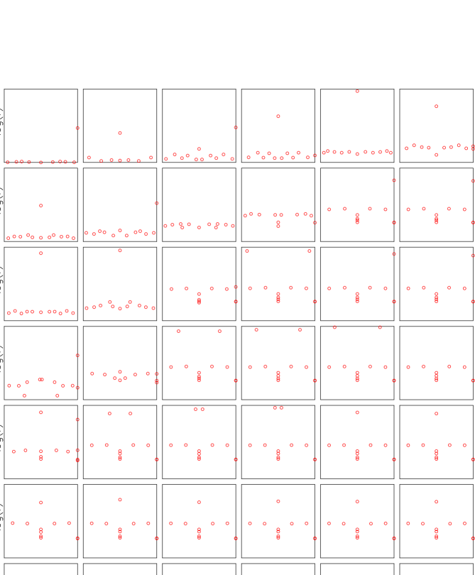
Figure 5: Leading spectrum of $\text{{{L}}}_{\epsilon}$ for different values of $\epsilon$ and $N$. If $\lambda_{i}$ is the $i$-th eigenvalue, then $\log\lambda_{i}=\log(r_{i})+{\rm i}\phi_{i}$ (where $r_{i}=|\lambda_{i}|$) and the coordinates in the plots are $(\phi,-\log(r))$. The ranges of the axes are $\phi\in[-\pi,\pi]$ and $-\log(r)\in[0,6]$. The map is the PAC with $k=0.02$ and the matrix was truncated to dim$=12$.

where $k$ is the small perturbation parameter. The map has a Lyapounov exponent which is almost independent of the value of $k$ and equal to $\lambda=\ln[(3+\sqrt{5})/2]$. On the other hand the Ruelle resonances (computed numerically) are very sensitive to it. Thus it is the ideal model to test the asymptotic results, independently of the short time Lyapunov regime. The map is a composition of two nonlinear shears and therefore it is easily quantized as a product of two noncommuting unitary operators. The explicit expression in the mixed representation is

$$\langle\,p\,|\hat{U}|\,q\,\rangle=\exp\left\{{\rm i}\frac{2\pi}{N}\left[\frac{q^{2}}{2}+qp-\frac{p^{2}}{2}\right]\right\}\times\mbox{\hskip 21.33955pt}$$

$$\mbox{\hskip 7.11317pt}\times\,\exp\Big{\{}2\pi N\,k\Big{(}\cos[2\pi q/N]+\cos[2\pi p/N]\Big{)}\Big{\}}$$ (65)

The other advantage of using a map of this type is that the propagation both of pure states and of density matrices can be done by fast Fourier techniques, thus allowing relatively large Hilbert spaces with reasonable CPU times. The minor disadvantage is that the quantization for this particular map is only valid for even values of $N$ hannay .

V.1 Spectrum

In Ref. garma we have performed the classical calculation of resonances and shown that the quantum and classical leading spectra coincide. Here we take a slightly different approach and just compute the quantum spectra for a range of $\epsilon$ and $N$ values, as shown in Fig. 5. Observe that there is an extended region where the spectrum is stable and independent of those parameters, signifying that the eigenvalues are properties exclusive of the map, and therefore coinciding with the classical resonances. It is clear from this figure that the limits $\epsilon\to 0$ and $N\to\infty$ cannot be independent. In fact, at fixed $N$ the limit $\epsilon\to 0$ restores unitarity and the spectrum returns to the unit circle.

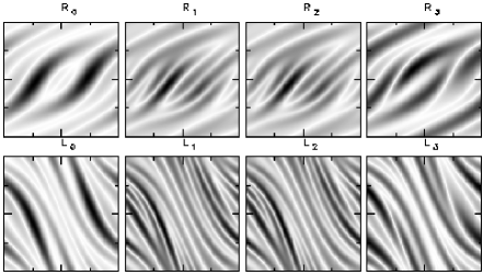
Figure 6: Top (bottom) row shows the first 4 right (left) eigenfunctions showing the unstable (stable) manifolds for the quantum PAC with $N=100$, $\epsilon=0.3$, $k=0.02$, and matrices truncated to dim$=12$.

Therefore, $\epsilon$ must decrease as a certain function of $N$. An optimal relationship between $N$ and $\epsilon$ is yet to be established but cannot be inferred from our limited data. However, in our range of values a dependence like $\epsilon\sim 1/\sqrt{N}$ seems suitable.

The method described in Sect. IV.2 also provides approximations to the eigenfunctions of $\text{{{L}}}_{\epsilon}$ corresponding to the leading eigenvalues. Inside the safe region (see Fig. 5) of $N$ and $\epsilon$ we were able to reconstruct at least 8 eigenfunctions successfully with matrices of dimension of order 12. The accuracy of these eigenfunctions was checked by evaluating the orthogonality properties in Eq. (38) and by computing the overlaps

$$\begin{array}[]{c}{1\over\lambda_{j}}(\,L_{i}\,|\text{{{L}}}_{\epsilon}|\,R_{j}\,)\\ {1\over\lambda_{j}}(\,R_{i}\,|\text{{{L}}}_{\epsilon}|\,L_{j}\,)\end{array}.$$ (66)

A plot of the absolute value of the Husimi representation for the first four eigenfunctions can be seen in Fig. 6. As was expected, the right (left) eigenfunctions corresponding to invariant densities of the propagator is smooth along the classical unstable (stable) manifold of the corresponding map. The right (left) eigenfunctions are not uniform along the unstable (stable) manifold showing pronounced peaks at the position of short periodic points. We intend to make a systematic analysis of this connection in a future work.

V.2 Asymptotic decay

In this section we study numerically the asymptotic behavior of the autocorrelation function, the linear entropy and the Loschmidt echo for the PAC. In Fig. 7 we see the growth of $C_{n}=-\ln[C(n)]$ and the growth of $S_{n}$ for the perturbed Arnold cat defined in Eq. (64) in Sect. V. In both cases there are two well defined regimes. Initially both grow with the slope determined by the Lyapunov exponent of the map. For the PAC the Lyapunov is essentially the same for a wide range of perturbations. On the other hand, the Ruelle resonances depend strongly on the perturbation. Taking as initial density a traceless pseudo-state (see Eq. (42)), time evolution of quantities show how the state approaches uniformity exponentially, with a rate given by the largest RP resonance. We observe that, after the Lyapunov regime (around the Eherenfest time $n_{E}$ ), the slope of the growth of $C_{n}$ is given by $\ln|\lambda_{1}|$ whereas the slope of $S_{n}$ is given by $2\ln|\lambda_{1}|$ as predicted. This factor two arises from the square in the definition of $S_{n}$ and is clearly seen in Fig. 7. The solid lines represent these two slopes and were obtained by computing $\lambda_{1}$ using the method described in Sec. IV.2.

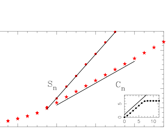
Figure 7: Purity decay and Correlation decay for the PAC (Eq. (64)) with $N=450$, $\epsilon=0.05$, $k=0.005$, initial pseudo-state $\hat{\rho}=|\,0,0\,\rangle\langle\,0,0\,|-\hat{I}/N$, where $|\,0,0\,\rangle$ is a coherent state centered at $(0,0)$. The inset shows the evolution of $S_{n}$ for $\hat{\rho}=|\,0,0\,\rangle\langle\,0,0\,|$ and how it saturates to the constant value $\ln N$.

In order to show the universality of the decay of the linear entropy and the Loschmidt echo, in terms of classical quantities, in Fig. 8 we show $S_{n}$ and $\ln(M_{n}(\epsilon))$ for various values of the parameter $\epsilon$. The linear entropy is simply the negative logarithm of the purity $\mbox{Tr}(\hat{\rho}_{n}^{2})$.

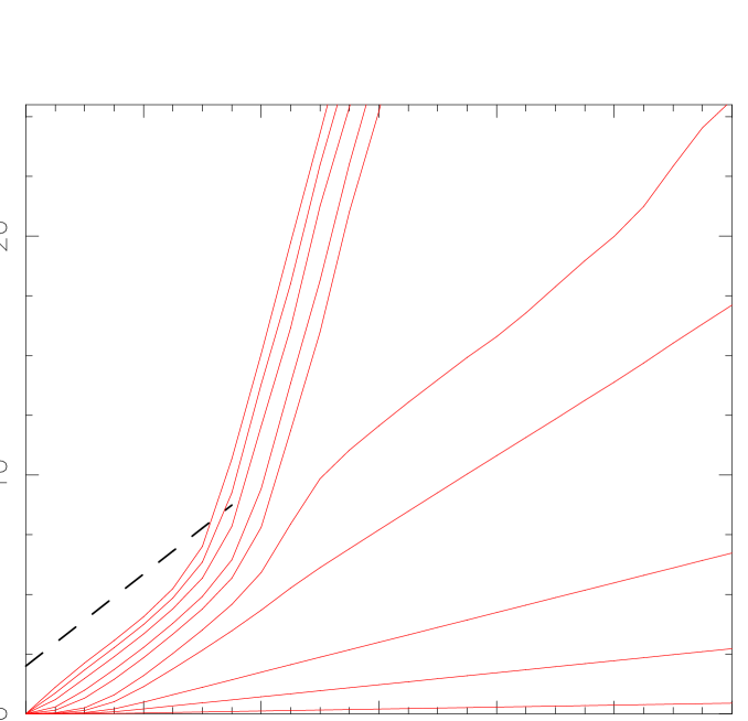
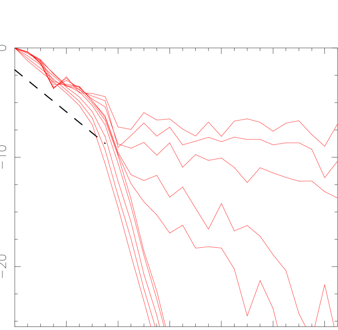
Figure 8: Linear entropy growth (left panel) and Loschmidt echo decay (right) for various values of $\epsilon$, ranging from $0.001$ to $0.1$ and for the PAC with $N=450$, $k=0.005$. Both Lyapunov and Ruelle regimes can be seen when the rates saturate at an $\epsilon$-independent value.

When $\epsilon\sim 0$ the purity is conserved and equal to one, so the linear entropy does not grow. However when $\epsilon\neq 0$ the purity will decay at a rate proportional to $\epsilon$. At one point, as predicted in zurek , the growth of the linear entropy saturates and no longer depends on $\epsilon$. Since we evolved a traceless pseudo-state, with no component on the uniform density, after the Lyapunov growth the Ruelle-Pollicot regime appears. In the same way as for the entropy, for small values of $\epsilon$ the asymptotic decay rate is $\epsilon$ dependent but it saturates when rate determined by the first Ruelle resonance is attained. This phenomenon can clearly be seen in Fig. 8 (left). In the right panel we display the echo and illustrate exactly the same feature.

VI Conclusions

We have developed a method to study numerically the spectral properties of open quantum maps on the torus. The method is particularly well suited to chaotic maps and provides reliable eigenvalues and eigenfunctions. The noise model that we implemented utilizes phase space translations as Kraus operators and is equivalent to coarse graining quantum Markovian master equations. Therefore it brings out classical properties of the map and we have shown that these properties are reflected in the asymptotic decay of several quantities. The same methods can be used to study other noise models in the context of quantum information theory, if one thinks of the quantum map as an algorithm to be implemented and the noise as the error source present in any implementation.

Appendix A Adjoint and linear action

Let ${\cal H}_{N}$ be a complex Hilbert space of dimension $N$. The space of linear operators acting on ${\cal H}_{N}$ is called Liouville space $\mathfrak{L}\equiv{\cal H}_{N^{2}}$. Elements in $\mathfrak{L}$ are usually represented by $N\times N$ dimensional complex matrices. However, given $\hat{A},\,\hat{B}\in{\cal H}_{N^{2}}$ then the “canonical” inner product, which induces the norm, is

$$(\hat{A},\hat{B})=\mbox{Tr}(\hat{A}^{\dagger}\hat{B}).$$ (67)

Thus ${\cal H}_{N^{2}}$ is a Hilbert space itself. Now, superoperators are a subset of the space of linear operators acting on ${\cal H}_{N^{2}}$. We introduce a bra-ket notation to simplify inner product expressions but also to distinguish the two types of decompositions we use for superopertors. Let $\hat{A},\,\hat{B}\in{\cal H}_{N^{2}}$ then the action of a superoperator $\text{{{S}}}:{\cal H}_{N^{2}}\to{\cal H}_{N^{2}}$ can be written as

$$\hat{B}=\text{{{S}}}(\hat{A})$$ (68)

or as

$$|\,B\,)=\text{{{S}}}|\,A\,)$$ (69)

indistinctly. The adjoint, in the bra-ket form, is defined as usual by

$$(\,A|\,\text{{{S}}}(\hat{B})\,)=(\,A|\text{{{S}}}|\,B\,)=(\,\text{{{S}}}^{\dagger}(\hat{A})|\,B\,),$$ (70)

which settles that $(\,A|\text{{{S}}}=(\,\text{{{S}}}^{{}^{\dagger}}(\hat{A})|$. Summarizing,

$$\begin{array}[]{rclcrcl}\hat{A}&\equiv&|\,A\,)&\mbox{\hskip 14.22636pt}&(\hat{A},\,\cdot\,)&\equiv&(\,A\,|\\ (\hat{A},\hat{B})&\equiv&(\,A|\,B\,)&\mbox{\hskip 14.22636pt}&\text{{{S}}}(\hat{A})&\equiv&\text{{{S}}}|\,A\,)\end{array}.$$ (71)

One way to think about it (not absolutely necessary but helpful) is to think of $\hat{A}$ as an operator, or matrix, in an operator space, acting on vectors, and $|\,A\,)$ as a vector in a vector space, acted on by superoperators.

Now, a completely positive superoperator has a Kraus operator sum representation. Suppose S is a completely positive supeorperator then there exist a set of operators $\{\hat{M}_{\mu}\}_{\mu=0}^{N^{2}-1}\in{\cal H}_{N^{2}}$, such that

$$\text{{{S}}}=\sum_{\mu}\hat{M}_{\mu}\otimes\hat{M}_{\mu}^{\dagger}$$ (72)

$\hat{M}_{\mu}$ are the Kraus operators. Without loss of generality, if the number of operators is smaller than $N^{2}$ we can always complete the set with zeros. The adjoint action of S on an operator $\hat{A}$ is defined through the Kraus representation suitable for the case of Eq. (68)

$$\text{{{S}}}(\hat{A})=\sum_{\mu}\hat{M}_{\mu}\hat{A}\hat{M}_{\mu}^{\dagger}.$$ (73)

Eq. (73) determines how the Kronecker product symbol $\otimes$ should be interpreted throughout this work.

On the other hand, a superoperator S can be written as an expansion of spectral projectors. Let $\hat{R}_{i}$ and $\hat{L}_{i}$ be right and left eigenoperators of L respectively, such that

$$\begin{array}[]{lll}\text{{{S}}}(\hat{R}_{i})&=&\lambda_{i}\hat{R_{i}}\\ \text{{{S}}}^{{}^{\dagger}}(\hat{L}_{i})&=&\lambda_{i}^{*}\hat{L_{i}}\end{array},\ \mbox{\hskip 28.45274pt}i=1,\ldots,N^{2},$$ (74)

and assume for simplicity that $\lambda_{i}$ are nondegenerate. Then the spectral projectors are

$$\hat{R}_{i}\,\mbox{Tr}(\hat{L}_{i}^{{}^{\dagger}},\,\cdot\,)=|\,R_{i}\,)(\,L_{i}|,$$ (75)

and the spectral decomposition is given by,

S $$= \sum_{i}|\,R_{i}\,)\lambda_{i}(\,L_{i}|$$ (76)

$$\text{{{S}}}^{\dagger} = \sum_{i}|\,L_{i}\,)\lambda_{i}^{*}(\,R_{i}|.$$ (77)

Therefore, given the spectral decomposition, the two ways of expressing the action of S on $\hat{A}$ are

$$\text{{{S}}}|\,A\,)=\sum_{i}|\,R_{i}\,)\lambda_{i}(\,L_{i}|\,A\,)\equiv\sum_{i}\hat{M}_{\mu}\hat{A}{\hat{M}_{\mu}}^{{}^{\dagger}}=\text{{{S}}}(\hat{A})$$ (78)

In more general terms Cavescaves identifies and describes the two different ways a superoperator acts as ordinary action (68) and left-right action (69). This provides two distinct decompositions of the same superoperator.

Appendix B Leading eigenvalues of a large matrix

In this section we describe in a general way the method used to compute the leading eigenvalues of the superoperator $\text{{{L}}}_{\epsilon}$ in section IV.2. It is based on the Lanczos power iteration methodgolub but was inspired by a recent work by Blum and Agam agam . This method is useful when only a few of the largest (in modulus) eigenvalues is needed and also, since it deals with large matrices, when there is an efficient subroutine to implement the matrix-vector product but there is no need to store the whole matrix in an array variable. Moreover, convergence and accuracy depends strongly on the distance part of the spectrum one wants to calculate and the part to be neglected.

In this work we don’t address the question of the estimation of errors.

Proposition 1

. Suppose $A$ is a large, sparse matrix in $\mathbb{C}^{n\times n}$ and assume each of its eigenvalues $\lambda_{i}$ has multiplicity one and that $1\geq|\lambda_{0}|>|\lambda_{1}|\ldots>|\lambda_{n-1}|$. Suppose $\left\{l_{i}\right\}_{i=0}^{n-1}$ and $\left\{r_{i}\right\}_{i=0}^{n-1}$ are the corresponding left and right eigenvectors

$$\mbox{\boldmath$A$}r_{i} = \lambda_{i}r_{i}$$ (79)

$$\mbox{\boldmath$A$}^{\dagger}l_{j} = \lambda^{*}_{j}l_{j},$$ (80)

and let $u_{0}\in\mathbb{C}^{n}$ be a vector such that

$$|(l_{i},u_{0})|>0\ \ \mbox{and}\ \ |(r_{i},u_{0})|>0\ \ \forall i<k$$ (81)

for some $k\leq n$, where $(\ ,\ )$ represents as usual the inner product. Then the first $k$ eigenvalues can be estimated from the reduced ($k\times k$) eigenvalue equation

$$\mbox{Det}\Big{[}\mbox{\boldmath$\cal K$}^{T}(\mbox{\boldmath$A$}^{\dagger},u_{0},k)\mbox{\boldmath$A$}\mbox{\boldmath$\cal K$}(\mbox{\boldmath$A$},u_{0},k)\mbox{\hskip 71.13188pt}$$

$$-z\mbox{\boldmath$\cal K$}^{T}(\mbox{\boldmath$A$}^{\dagger},u_{0},k)\mbox{\boldmath$\cal K$}(\mbox{\boldmath$A$},u_{0},k)\Big{]}=0$$ (82)

where $\mbox{\boldmath$\cal K$}(\mbox{\boldmath$A$},u_{0},k)$ is the Krylov matrix whose columns are the iterates of $u_{0}$,

$$\mbox{\boldmath$\cal K$}(\mbox{\boldmath$A$},u_{0},k)=\left[u_{0},\mbox{\boldmath$A$}u_{0},\mbox{\boldmath$A$}^{2}u_{0},\ldots,\mbox{\boldmath$A$}^{k-1}u_{0}\right]$$ (83)

and ^T as usual denotes matrix transposition.

Proof. We sketch a rather straightforward proof (though perhaps not entirely rigorous). The sets $\left\{l_{i}\right\}_{i=0}^{n-1}$ and $\left\{r_{i}\right\}_{i=0}^{n-1}$ of left and right eigenvectors of $A$ are complete and, they can be normalized according to

$$(l_{i},r_{j})=\delta_{ij}.$$ (84)

Therefore there exist two distinct expansions of $u_{0}$

$$u_{0} = \sum_{i=0}^{n-1}\alpha_{i}\,r_{i}$$ (85)

$$u_{0} = \sum_{i=0}^{n-1}\beta_{i}\,l_{i}.$$ (86)

In terms of these expansions we obtain

$$\mbox{\boldmath$\cal K$}^{T}(\mbox{\boldmath$A$}^{\dagger},u_{0},k)\mbox{\boldmath$\cal K$}(\mbox{\boldmath$A$},u_{0},k)=\left[\begin{array}[]{c}\sum_{i}\beta_{i}\,l_{i}\\ \sum_{i}\beta_{i}\lambda_{i}^{*}\,l_{i}\\ \vdots\\ \sum_{i}\beta_{i}\lambda_{i}^{*^{k-1}}\,l_{i}\end{array}\right]\ \left[\sum_{j}\alpha_{j}\,r_{j},\sum_{j}\alpha_{j}\lambda_{j}\,r_{j},\cdots,\sum_{j}\alpha_{j}\lambda_{j}^{k-1}\,r_{j}\right]$$ (87)

which yields

$$\left[\mbox{\boldmath$\cal K$}^{T}(\mbox{\boldmath$A$}^{\dagger},u_{0},k)\mbox{\boldmath$\cal K$}(\mbox{\boldmath$A$},u_{0},k)\right]_{\mu\nu} = \sum_{i,j}\alpha_{j}\beta_{i}\lambda_{j}^{\nu}\lambda_{i}^{*^{\mu}}(l_{i},r_{j})$$ (88)

$$= \sum_{i}\alpha_{i}\beta_{i}\lambda_{i}^{\nu}\lambda_{i}^{*^{\mu}},$$

and similarly

$$\left[\mbox{\boldmath$\cal K$}^{T}(\mbox{\boldmath$A$}^{\dagger},u_{0},k)\mbox{\boldmath$A$}\mbox{\boldmath$\cal K$}(\mbox{\boldmath$A$},u_{0},k)\right]_{\mu\nu} = \sum_{i,j}\beta_{i}\alpha_{j}\lambda_{j}^{\nu+1}\lambda_{i}^{*^{\mu}}(l_{i},r_{j})$$ (89)

$$= \sum_{i}\beta_{i}\alpha_{i}\lambda_{i}^{\nu+1}\lambda_{i}^{*^{\mu}}.$$

Thus, Eq. (82) can be re-written as

$$\mbox{Det}\left[\sum_{i=0}^{n-1}\alpha_{i}\beta_{i}\lambda_{i}^{\nu}\lambda_{i}^{*^{\mu}}(\lambda_{i}-z)\right]=0.$$ (90)

If all the conditions of the proposition are met, this equation is equivalent to the original full eigenvalue equation. Now, since $\lambda_{i}$ are ordered by dereasing modulus and assuming that the eigenvalues accumulate around zero, leaving only a few, say $k$ of them, with significant modulus (as is the case for the maps studied in section IV.2) then we can neglect the contribution of the last $n-k$ terms in the sum. Thus Eq. (90) is just the determinant of the product of three $k\times k$ square matrices

$$\mbox{Det}[\mbox{\boldmath$\Lambda$}^{\dagger}\,\mbox{\boldmath$\Xi\,\Lambda$}]=\mbox{Det}[\mbox{\boldmath$\Lambda$}^{\dagger}]\,\mbox{Det}[\mbox{\boldmath$\Xi$}]\,\mbox{Det}[\mbox{\boldmath$\Lambda$}]=0$$ (91)

where

$$\mbox{\boldmath$\Lambda$}=\left(\begin{array}[]{ccccc}1&\lambda_{0}&\lambda_{0}^{2}&\cdots&\lambda_{0}^{k-1}\\ 1&\lambda_{1}&\lambda_{1}^{2}&\cdots&\lambda_{1}^{k-1}\\ \vdots&\vdots&\vdots&\ddots&\vdots\\ 1&\lambda_{k-1}&\lambda_{k-1}^{2}&\cdots&\lambda_{k-1}^{k-1}\end{array}\right);\mbox{\hskip 21.33955pt}\mbox{\boldmath$\Xi$}=\left(\begin{array}[]{cccc}\alpha_{0}\beta_{0}(\lambda_{0}-z)&0&\cdots&0\\ 0&\alpha_{1}\beta_{1}(\lambda_{1}-z)&\cdots&0\\ \vdots&\vdots&\ddots&\vdots\\ 0&\cdots&0&\alpha_{k-1}\beta_{k-1}(\lambda_{k-1}-z)\end{array}\right).$$ (92)

The matrix $\Lambda$ is a Vandermonde matrix. The determinant of a Vandermonde matrix $\mbox{\boldmath$\Lambda$}_{k}(\lambda_{0},\ldots,\lambda_{k-1})$ is given by

$$\mbox{Det}\left[\mbox{\boldmath$\Lambda$}_{k}(\lambda_{0},\ldots,\lambda_{k-1})\right]=\prod_{0\leq i\leq j\leq k-1}(\lambda_{j}-\lambda_{i}).$$ (93)

From equation Eq. (93) it can be readily seen that if the spectrum of $A$ is non-degenerate then $\Lambda$ is invertible. Moreover, the structure of $\Lambda$ determines $k$ because in the limit of $k$ “too large”, $\Lambda$ is singular, at least to within computing precision. So, using properties of the determinant in the secular equation Eq. (91), we get

$$\mbox{Det}[\mbox{\boldmath$\Xi$}]=\prod_{\mu}\alpha_{\mu}\beta_{\mu}(\lambda_{\mu}-z)=0.$$ (94)

Since, from the hypothesis, $\alpha_{\mu}\beta_{\mu}\neq 0$ then Eq. (94) yields the desired solution, i.e. the first $k$ eigenvalues of $A$. $\square$

In practice, the usefulness of the method depends upon the gap $(1-|\lambda_{1}|)$, because it determines how fast the terms of the sum in Eq. (91) decay.

In section IV.2 the span of the sets ${\cal F}$ and ${\cal B}$ are just the Krylov spacesgolub of $\text{{{L}}}_{\epsilon}$ and $\text{{{L}}}_{\epsilon}^{\dagger}$, and using the present notation Eq. (63) is

$$\mbox{Det}\Big{[}\mbox{\boldmath$\cal K$}^{\dagger}(\text{{{L}}}_{\epsilon}^{\dagger},\hat{\rho}_{0},n_{\text{max}})\text{{{L}}}_{\epsilon}\mbox{\boldmath$\cal K$}(\text{{{L}}}_{\epsilon},\hat{\rho}_{0},n_{\text{max}})\mbox{\hskip 56.9055pt}$$

$$-z\,\mbox{\boldmath$\cal K$}^{\dagger}(\text{{{L}}}_{\epsilon}^{\dagger},\hat{\rho}_{0},n_{\text{max}})\mbox{\boldmath$\cal K$}(\text{{{L}}}_{\epsilon},\hat{\rho}_{0},n_{\text{max}})\Big{]}=0\mbox{\hskip 14.22636pt}$$ (95)

In analogy with Eq. (91). The efficiency of this method depends strongly on the spectrum configuration. The case of the coarse-grained propagator of hyperbolic maps on the torusblank ; nonn is particularly favorable because of the significant gap between 1 and $\lambda_{1}$ and because 0 is an accumulation point, so a large number of resonances can be discarded and the size of the matrices is reduced dramatically.

References

- (1) See e.g M. Brack and R. K. Bhaduri “Semiclassical Physics”, Addison-Weseley, Reading, MA (1997).
- (2) M. C. Gutzwiller, “Chaos in Classical and Quantum Mechanics”. Springer-Verlag, New York (1990).
- (3) W. H. Zurek and J. P. Paz, Phys. Rev. Lett 72, 2508 (1994).
- (4) A. Peres. Phys, Rev A 30, 1610 (1984).
- (5) R. A. Jalabert and H. M. Pastawski, Phys. Rev. Lett. 86,2490 (2001); Ph. Jaquod, P. G. Silverstrov and C. W. J. Beenakker, Phys. Rev. E 64 055203(R) (2001); F. M. Cucchietti, H. M. Pastawski, and D. A. Wisniacki, Phys. Rev. E, 65,045206 (2002); G. Benenti and G. Casati. Phys. Rev. E 65, 066205 (2002).
- (6) T. Prosen and M. Znidaric, J. Phys. A 34, L681 (2001); T. Prosen, Phys. Rev. E 65, 036208 (2002).
- (7) A. Jordan and M. Srednicki. Preprint, nlin.CD/0108024.
- (8) I. García-Mata, M. Saraceno, and M. E. Spina, Phys. Rev. Lett. 91, 064101 (2003).
- (9) D. Ruelle, Phys. Rev. Lett. 56, 405 (1986); D. Ruelle, J. Stat. Phys 44, 281 (1986).
- (10) K. Pance, W. T. Lu and S. Sridhar, Phys. Rev. Lett. 85, 2737 (2000).
- (11) C. Manderfeld, J. Weber, and F. Haake, J. Phys. A 34, 9893 (2001).
- (12) J. Weber, F. Haake, and P. Seba, Phys. Rev. Lett. 85, 3620-3623 (2000).
- (13) D. Braun, CHAOS, 9,730 (1999) and D. Braun, Physica D, 131, 265 (1999).
- (14) S. Fishman, Wave Functions, Wigner Functions and Green Functions of Chaotic Systems in “Supersymmetry and Trace Formulae Chaos and Disorder”, NATO ASI Series, edited by I. V. Lerner, J. P. Keating and D. E. Khmelnitskii. (Kluwer Academic/Plenum Publishers, New York, 1999).
- (15) M. Khodas, S. Fishman, and O. Agam. Phys. Rev. E. 62, 4769 (2000); S. Fishman and S. Rahav, nlin.CD/0204068.
- (16) H. H. Hasegawa and W. C. Saphir, Phys. Rev. A 46, 7401 (1992).
- (17) M. Blank, G. Keller, and C. Liverani, Nonlinearity 15, pp.1905-1973 (2002).
- (18) S. Nonnenmacher, Nonlinearity 16, pp.1685-1713 (2003).
- (19) A.M. Ozorio de Almeida Phys. Rep. 295 266 (1998); A. Rivas and A. M. Ozorio de Almeida, Ann. Phys. (N.Y.)276, 223 (1999).
- (20) C. Miquel, J. P. Paz and M. Saraceno, Phys. Rev. A, 65, 2309 (2002).
- (21) J. Schwinger, Proc. Nat. Acad. Sci. 46, 570 (1960).
- (22) A. M. Ozorio de Almeida, “Hamiltonian Systems: Chaos and Quantization”. Cambridge University Press, Cambridge (1988).
- (23) J. H. Hannay and M. V. Berry, Physica 1D,267-290 (1980).
- (24) M. Basilio de Matos and A. M. Ozorio de Almeida, Ann. Phys. 237, 46-65 (1995)
- (25) M. L. Balazs and A. Voros, Ann. Phys. 190,1 (1989).
- (26) M. Saraceno, Ann. Phys. 99, 37 (1990).
- (27) F. M. Izrailev, Phys. Rev. Lett. 56, 541 (1986).
- (28) M. V. Berry, N. L. Balazs, M. Tabor and A. Voros, Ann. Phys. N. Y. 122, 26 (1979).
- (29) W. H. Zurek, Rev. Mod. Phys. 75, pp. 715-775 (2003).
- (30) J. P. Paz, and W. H. Zurek, in Coherent Matter Waves, Les Houches Session LXXII,1999, edited by R. Kaiser, C. Westbrook, and F. David (EDP Sciences, Springer-Verlag, Berlin 2001).
- (31) G. W. Gardiner and P. Zoller, “Quantum Noise: A Handbook of Markovian and Non-Markovian Quantum Stochastic Methods with Applications to Quantum Optics”, Springer-Verlag, Berlin-Heidelberg 2000.
- (32) B. Kümmerer. Quantum Markov Processes in “Coherent Evolution in Noisy Environments”, A. Buchleitner and K. Hornberger (Eds.), Springer-Verlag, Berlin-Heidelberg (2002).
- (33) G. Lindblad, Commun. Math Phys, 48, 119 (1976).
- (34) I. Percival Quantum State Diffusion (1998). (Cambridge: Cambridge University Press).
- (35) K. Kraus, States, Effects and Operations, Springer-Verlag, Berlin, 1983.
- (36) J. Preskill. “1998 Lecture Notes for Physics 229: Quantum Information and Computation” available at http://www.theory.caltech.edu/people/preskill.
- (37) I. Chuang and M. Nielsen. Quantum Information and Computation (Cambridge University Press, Cambridge, UK, 2001).
- (38) B. Schumacher, Phys. Rev. A 54, 2814 (1996).
- (39) C. M. Caves, Journal of Superconductivity 12, 707-718 (1999).
- (40) P. Bianucci, J. P. Paz, and M. Saraceno, Phys. Rev. E 65, 046226 (2002).
- (41) See, for example, P. Gaspard, “Chaos Scattering and Statistical Mechanics”, Cambirdge Nonlinear Science Series 9, Cambirdge University Press, Cambridge (1998).
- (42) G. Palla, G. Vattay and Andre Voros, Phys. Rev. E 64, 012104 (2001); D. Braun, “Dissipative Quantum Chaos and Decoherence”, Springer-Verlag, Berlin-Heidelberg (2001).
- (43) H. H. Rugh, Nonlinearity 5, 1237-1263 (1992).
- (44) G. Blum and O. Agam, Phys. Rev. E 62, 1977 (2000).
- (45) R. Florido, J. M. Martín-González and J. M. Gómez Llorente, Phys. Rev. E 66, 046208 (2002).
- (46) A. K. Pattanayak, Phys. Rev. Lett., 83, 4526 (1999).
- (47) D. Monteoliva and J. P. Paz, Phys. Rev. Lett 85, 3373 (2000).
- (48) T. F. Havel, J. Math. Phys. 44, 534 (2003).
- (49) G. H. Golub, and Charles F. Van Loan. “Matrix Computations”, The Johns Hopkins University Press, Baltimore (1996).