Quantum and Arithmetical Chaos

Abstract

The lectures are centered around three selected topics of quantum chaos: the Selberg trace formula, the two-point spectral correlation functions of Riemann zeta function zeros, and of the Laplace–Beltrami operator for the modular group. The lectures cover a wide range of quantum chaos applications and can serve as a non-formal introduction to mathematical methods of quantum chaos.

Introduction

Quantum chaos is a nickname for the investigation of quantum systems which do not permit exact solutions. The absence of explicit formulas means that underlying problems are so complicated that they cannot be expressed in terms of known ($\simeq$ simple) functions. The class of non-soluble systems is very large and practically any model (except a small set of completely integrable systems) belongs to it. An extreme case of quantum non-soluble problems appears naturally when one considers the quantization of classically chaotic systems which explains the word ‘chaos’ in the title.

As, by definition, for complex systems exact solutions are not possible, new analytical approaches were developed within the quantum chaos. First, one may find relations between different non-integrable models, hoping that for certain questions a problem will be more tractable than another. Second, one considers, instead of exact quantities, the calculation of their smoothed values. In many cases such coarse graining appears naturally in experimental settings and, usually, it is more easy to treat. Third, one tries to understand statistical properties of quantum quantities by organizing them in suitable ensembles. An advantage of such approach is that many different models may statistically be indistinguishable which leads to the notion of statistical universality.

The ideas and methods of quantum chaos are not restricted only to quantum models. They can equally well be applied to any problem whose analytical solution either is not possible or is very complicated. One of the most spectacular examples of such interrelations is the application of quantum chaos to number theory, in particular, to the zeros of the Riemann zeta function. Though a hypothetical quantum-like system whose eigenvalues coincide with the imaginary part of Riemann zeta function zeros is not (yet!) found, the Riemann zeta function is, in many aspects, similar to dynamical zeta functions and the investigation of such relations already mutually enriched both quantum chaos and number theory (see e.g. the calculation by Keating and Snaith moments of the Riemann zeta function using the random matrix theory KeatingSnaith ).

The topics of these lectures were chosen specially to emphasize the interplay between physics and mathematics which is typical for quantum chaos.

In Chap. 1 different types of trace formulas are discussed. The main attention is given to the derivation of the Selberg trace formula which relates the spectral density of automorphic Laplacian on hyperbolic surfaces generated by discrete groups with classical periodic orbits for the free motion on these surfaces. This question is rarely discussed in the physical literature but is of general interest because it is the only case where the trace formula is exact and not only a leading semiclassical contribution as for general dynamical systems. Short derivations of trace formulas for dynamical systems and for the Riemann zeta function zeros are also presented in this Chapter.

According to the well-known conjecture BohigasGiannoni statistical properties of eigenvalues of energies of quantum chaotic systems are described by standard random matrix ensembles depending only on system symmetries. In Chap. 2 we discuss analytical methods of confirmation of this conjecture. The largest part of this Chapter is devoted to a heuristic derivation of the ‘exact’ two-point correlation function for the Riemann zeros. The derivation is based on the Hardy–Littlewood conjecture about the distribution of prime pairs which is also reviewed. The resulting formula agrees very well with numerical calculations of Odlyzko.

In Chap. 3 a special class of dynamical systems is considered, namely, hyperbolic surfaces generated by arithmetic groups. Though from viewpoint of classical mechanics these models are the best known examples of classical chaos, their spectral statistics are close to the Poisson statistics typical for integrable models. The reason for this unexpected behavior is found to be related with exponential degeneracies of periodic orbit lengths characteristic for arithmetical systems. The case of the modular group is considered in details and the exact expression for the two-point correlation function for this problem is derived.

To be accessible for physics students the lectures are written in a non-formal manner. In many cases analogies are used instead of theorems and complicated mathematical notions are illustrated by simple examples.

Chapter 1 Trace Formulas

Different types of trace formula are the cornerstone of quantum chaos. Trace formulas relate quantum properties of a system with its classical counterparts. In the simplest and widely used case the trace formula expresses the quantum density of states through a sum over periodic orbits and each term in this sum can be calculated from pure classical mechanics.

In general, dynamical trace formulas represent only the leading term of the semiclassical expansion in powers of $\hbar$. The computation of other terms is possible though quite tedious Gaspard . The noticeable exception is the free motion on constant negative curvature surfaces generated by discrete groups where the trace formula (called the Selberg trace formula) is exact. The derivation of this formula is the main goal of this Section.

For clarity, in Sect. 1 the simplest case of the rectangular billiard is briefly considered and the trace formula for this system is derived. The derivation is presented in a manner which permits to generalize it to the Selberg case of constant negative curvature surfaces generated by discrete groups which is considered in details in Sect. 2. In Sects. 3 and 4 the derivations of the trace formula for, respectively, classically integrable and chaotic systems are presented. In Sect. 5 it is demonstrated that the density of Riemann zeta function zeros can be written as a sort of trace formula where the role of periodic orbits is played by prime numbers. Section 6 is the summary of this Chapter.

1 Plane Rectangular Billiard

To clarify the derivation of trace formulas let us consider in details a very simple example, namely, the computation of the energy spectrum for the plane rectangular billiard with periodic boundary conditions.

This problem consists of solving the equation

$$(\varDelta+E_{\vec{n}})\Psi_{\vec{n}}(x,y)=0$$ (1.1)

where $\varDelta=\partial^{2}/\partial x^{2}+\partial^{2}/\partial y^{2}$ is the usual two-dimensional Laplacian with periodic boundary conditions

$$\Psi_{\vec{n}}(x+a,y)=\Psi_{\vec{n}}(x,y+b)=\Psi_{\vec{n}}(x,y)$$ (1.2)

where $a$ and $b$ are sizes of the rectangle.

The plane wave

$$\Psi_{\vec{n}}(x,y)=e^{{\rm i}k_{1}x+{\rm i}k_{2}y}$$

is an admissible solution of (1.1). Boundary conditions (1.2) determine the allowed values of the momentum $\vec{k}$

$$k_{1}=\frac{2\pi}{a}n_{1},\;\;\;\;k_{2}=\frac{2\pi}{b}n_{2}\;,$$

with $n_{1},n_{2}=0,\pm 1,\pm 2,\ldots$, and, consequently, energy eigenvalues are

$$E_{n_{1}n_{2}}=\left(\frac{2\pi}{a}n_{1}\right)^{2}+\left(\frac{2\pi}{b}n_{2}\right)^{2}\;.$$ (1.3)

The first step of construction of trace formulas is to consider instead of individual eigenvalues their density defined as the sum over all eigenvalues which explains the word ‘trace’

$$d(E)\equiv\sum_{n_{1},n_{2}=-\infty}^{+\infty}\delta(E-E_{n_{1}n_{2}})\;.$$ (1.4)

To transforms this and similar expressions into a convenient form one often uses the Poisson summation formula

$$\sum_{n=-\infty}^{+\infty}f(n)=\sum_{m=-\infty}^{+\infty}\int_{-\infty}^{+\infty}\mathrm{e}^{2\pi{\rm i}mn}f(n)\mathrm{d}n\;.$$ (1.5)

An informal proof of this identity can, for example, be done as follows.

First

$$\sum_{n=-\infty}^{+\infty}f(n)=\int_{-\infty}^{+\infty}f(x)g(x)\mathrm{d}x$$

where $g(x)$ is the periodic $\delta$-function

$$g(x)=\sum_{m=-\infty}^{+\infty}\delta(x-n)\;.$$

As any periodic function with period 1, $g(x)$ can be expanded into the Fourier series

$$g(x)=\sum_{m=-\infty}^{+\infty}\mathrm{e}^{2\pi{\rm i}mx}c_{m}\;.$$

Coefficients $c_{m}$ are obtained by the integration of $g(x)$ over one period

$$c_{m}=\int_{-1/2}^{+1/2}g(y)\mathrm{e}^{-2\pi{\rm i}my}\mathrm{d}y=1$$

which gives (1.5).

By applying the Poisson summation formula (1.5) to the density of states (1.4) one gets

$$d(E) = \sum_{m_{1},m_{2}=-\infty}^{+\infty}\int\int\mathrm{e}^{2\pi{\rm i}(m_{1}n_{1}+m_{2}n_{2})}\times$$

$$\times \delta\left(E-\left(\frac{2\pi}{a}n_{1}\right)^{2}-\left(\frac{2\pi}{b}n_{2}\right)^{2}\right)\mathrm{d}n_{1}\mathrm{d}n_{2}\;.$$

Perform the following substitutions: $E=k^{2}$, $n_{1}=ar\cos\varphi/2\pi$, and $n_{2}=br\sin\varphi/2\pi$. Then $\mathrm{d}n_{1}\mathrm{d}n_{2}=abr\mathrm{d}r\mathrm{d}\varphi/(2\pi)^{2}$ and

$$d(E) = \frac{\mu(D)}{(2\pi)^{2}}\sum_{m_{1},m_{2}=-\infty}^{+\infty}\int\int\mathrm{e}^{{\rm i}(m_{1}a\cos\varphi+m_{2}b\sin\varphi)r}\delta(k^{2}-r^{2})r\mathrm{d}r\mathrm{d}\varphi$$

$$= \frac{\mu(D)}{2(2\pi)^{2}}\sum_{m_{1},m_{2}=-\infty}^{+\infty}\int_{0}^{2\pi}\mathrm{e}^{{\rm i}k\sqrt{(m_{1}a)^{2}+(m_{2}b)^{2}}\cos\varphi}\mathrm{d}\varphi$$

$$= \frac{\mu(D)}{4\pi}\sum_{m_{1},m_{2}=-\infty}^{+\infty}J_{0}(kL_{p})\;,$$

where $\mu(D)=ab$ is the area of the rectangle,

$$J_{0}(x)=\frac{1}{2\pi}\int_{0}^{2\pi}\mathrm{e}^{{\rm i}x\cos\varphi}\mathrm{d}\varphi$$

is the Bessel function of order zero (see e.g. Bateman , Vol. 2, Sect. 7), and

$$L_{p}=\sqrt{(m_{1}a)^{2}+(m_{2}b)^{2}}$$

is (as it is easy to check) the length of a periodic orbit in the rectangle with periodic boundary conditions.

Separating the term with $m_{1}=m_{2}=0$ one concludes that the eigenvalue density of the rectangle with periodic boundary conditions can be written as the sum of two terms

$$d(E)=\bar{d}(E)+d^{(osc)}(E)\;,$$

where

$$\bar{d}(E)=\frac{\mu(D)}{4\pi}$$ (1.6)

is the smooth part of the density and

$$d^{(osc)}(E)=\frac{\mu(D)}{4\pi}\sum_{\mbox{p.o.}}J_{0}(kL_{p})\;,$$ (1.7)

is the oscillating part equal to a sum over all periodic orbits in the rectangle.

As

$$J_{0}(z)\stackrel{{\scriptstyle z\to\infty}}{{\longrightarrow}}\sqrt{\frac{2}{\pi z}}\cos\left(z-\frac{\pi}{4}\right)$$

the oscillating part of the level density in the semiclassical limit $k\to\infty$ takes the form

$$d^{(osc)}(E)=\frac{\mu(D)}{\sqrt{8\pi k}}\sum_{\mbox{p.o.}}\frac{1}{\sqrt{L_{p}}}\cos\left(kL_{p}-\frac{\pi}{4}\right)\;.$$ (1.8)

Let us repeat the main steps which lead to this trace formula. One starts with an explicit formula (like (1.3)) which expresses eigenvalues as a function of integers. Using the Poisson summation formula (1.5) the density of states (1.4) is transformed into a sum over periodic orbits. In Sect. 3 it will be demonstrated that exactly this method can be applied for any integrable systems in the semiclassical limit where eigenvalues can be approximated by the WKB formulas.

More Refined Approach

The above method of deriving the trace formula for the rectangular billiard can be applied only if one knows an explicit expression for eigenvalues. For chaotic systems this is not possible and another method has to be used.

Assume that one has to solve the equation

$$(E_{\vec{n}}-\hat{H})\Psi_{\vec{n}}(\vec{x})=0$$

for a certain problem with a Hamiltonian $\hat{H}$. Under quite general conditions eigenfunctions $\Psi_{\vec{n}}(\vec{x})$ can be chosen orthogonal

$$\int\Psi_{\vec{n}}(\vec{x})\Psi_{\vec{m}}^{*}(\vec{x})\mathrm{d}\vec{x}=\delta_{nm}$$

and they form a complete system of functions

$$\sum_{\vec{n}}\Psi_{\vec{n}}(\vec{x})\Psi_{\vec{n}}^{*}(\vec{y})=\delta(\vec{x}-\vec{y})\;.$$

The Green function of the problem, by definition, obeys the equation

$$(E-\hat{H})G_{E}(\vec{x},\vec{y})=\delta(\vec{x}-\vec{y})$$

and the same boundary conditions as the original eigenfunctions. Its explicit form can formally be written through exact eigenfunctions and eigenvalues as follows

$$G_{E}(\vec{x},\vec{y})=\sum_{\vec{n}}\frac{\Psi_{\vec{n}}(\vec{x})\Psi_{\vec{n}}^{*}(\vec{y})}{E-E_{n}+{\rm i}\epsilon}\;.$$ (1.9)

The $+{\rm i}\epsilon$ prescription determines the so-called retarded Green function.

Example

To get used to Green functions let us consider in details the calculation of the Green function for the free motion in $f$-dimensional Euclidean space. This Green function obeys the free equation

$$(E+\hbar^{2}\varDelta)G_{E}^{(0)}(\vec{x},\vec{y})=\delta(\vec{x}-\vec{y})\;.$$ (1.10)

Let us look for the solution of the above equation in the form $G_{E}^{(0)}(\vec{x},\vec{y})=G(r)$ where $r=|\vec{x}-\vec{y}|$ is the distance between two points.

Simple calculations shows that for $r\neq 0$ $G(r)$ obeys the equation

$$\frac{\mathrm{d}^{2}G}{\mathrm{d}r^{2}}+\frac{f-1}{r}\frac{\mathrm{d}G}{\mathrm{d}r}+\frac{k^{2}}{\hbar^{2}}G=0$$

where $E=k^{2}$.

After the substitution

$$G(r)=r^{1-f/2}g\left(\frac{k}{\hbar}r\right)$$

one gets for $g(z)$ the Bessel equation (see e.g. Bateman , Vol. 2, Sect. 7)

$$\frac{\mathrm{d}^{2}g}{\mathrm{d}z^{2}}+\frac{1}{z}\frac{\mathrm{d}g}{\mathrm{d}z}+\left(1-\frac{\nu^{2}}{z^{2}}\right)g=0$$ (1.11)

with $\nu=|f/2-1|$.

There are many solutions of this equation. The above $+{\rm i}\epsilon$ prescription means that when $k\to k+i\epsilon$ with a positive $\epsilon$ the Green function has to decrease at large distances. It is easy to see that $G(r)$ is proportional to $\mathrm{e}^{\pm{\rm i}kr/\hbar}$ at large $r$. The $+i\epsilon$ prescription selects a solution which behaves at infinity like $\mathrm{e}^{+{\rm i}kr/\hbar}$ with positive $k$. The required solution of (1.11) is the first Hankel function (see Bateman , Vol. 2, Sect. 7)

$$g(z)=C_{f}H_{\nu}^{(1)}(z)$$ (1.12)

where $C_{f}$ is a constant and $H_{\nu}^{(1)}(z)$ has the following asymptotics for large and small $z$

$$H_{\nu}^{(1)}(z)\stackrel{{\scriptstyle z\to\infty}}{{\longrightarrow}}\sqrt{\frac{2}{\pi z}}\mathrm{e}^{{\rm i}(z-\pi\nu/2-\pi/4)}$$

and

$$H_{\nu}^{(1)}(z)\stackrel{{\scriptstyle z\to 0}}{{\longrightarrow}}\left\{\begin{array}[]{cl}-{\rm i}2^{\nu}\Gamma(\nu)z^{-\nu}/\pi\;,&\;\nu\neq 2\\ 2{\rm i}\ln z/\pi\;,&\;\nu=2\end{array}\right.\;.$$

The overall factor in (1.12) has to be computed from the requirement that the Green function will give the correct $\delta$-function contribution in the right hand side of (1.10). This term can appear only in the result of differentiation of the Green function at small $r$ where it has the following behaviour

$$G(r)\stackrel{{\scriptstyle r\to 0}}{{\longrightarrow}}G_{0}(r)=A_{f}r^{2-f}$$

with

$$A_{f}=C_{f}\frac{2^{\nu}\hbar^{\nu}\Gamma(\nu)}{{\rm i}\pi k^{\nu}}\;.$$

One should have

$$\hbar^{2}\varDelta G_{0}(r)=\delta(\vec{r})\;.$$ (1.13)

Multiplying this equality by a suitable test function $f(r)$ quickly decreasing at infinity one has

$$\hbar^{2}\int f(r)\varDelta G_{0}(r)\mathrm{d}\vec{r}=f(0)\;.$$

Integrating by parts one obtains

$$\hbar^{2}\int\frac{\partial}{\partial x_{\mu}}f(r)\frac{\partial}{\partial x_{\mu}}G_{0}(r)\mathrm{d}\vec{r}=-f(0)\;.$$

As both functions $f(r)$ and $G_{0}(r)$ depend only on the modulus of $\vec{r}$ one finally finds

$$\hbar^{2}\int_{0}^{\infty}\frac{\mathrm{d}f(r)}{\mathrm{d}r}\frac{\mathrm{d}G_{0}(r)}{\mathrm{d}r}r^{f-1}\mathrm{d}rS_{f-1}=-f(0)$$

where $S_{f-1}$ is the volume of the $(f-1)$-dimensional sphere $x_{1}^{2}+\ldots+x_{f}^{2}=1$. Using (1.13) one concludes that in order to give the $\delta$-function term $A_{f}$ has to obey

$$\hbar^{2}A_{f}(f-2)S_{f-1}=-1\;.$$

One of the simplest method of calculation of $S_{f-1}$ is the following identity

$$\int_{-\infty}^{\infty}\mathrm{e}^{-x_{1}^{2}}\mathrm{d}x_{1}\int_{-\infty}^{\infty}\mathrm{e}^{-x_{2}^{2}}\mathrm{d}x_{2}\ldots\int_{-\infty}^{\infty}\mathrm{e}^{-x_{f}^{2}}\mathrm{d}x_{f}=\pi^{f/2}\;.$$

By changing Cartesian coordinates in the left hand side to hyper-spherical ones we obtain

$$\int_{0}^{\infty}\mathrm{e}^{-r^{2}}r^{f-1}\mathrm{d}rS_{f-1}=\pi^{f/2}$$

which gives

$$S_{f-1}=\frac{2\pi^{f/2}}{\Gamma(f/2)}$$

where $\Gamma(x)$ is the usual gamma-function (see e.g. Bateman , Vol. 1, Sect. 1).

Combining together all terms and using the relation $x\Gamma(x)=\Gamma(x+1)$ one gets the explicit expression for the free Green function in $f$ dimensions

$$G^{(0)}_{E}(\vec{x},\vec{y})=\frac{k^{\nu}}{4i\hbar^{2}(2\pi\hbar r)^{\nu}}H_{\nu}^{(1)}\left(\frac{k}{\hbar}|\vec{x}-\vec{y}|\right)$$ (1.14)

where $\nu=|f/2-1|$. In particular, in the two-dimensional Euclidean space

$$G^{(0)}_{E}(\vec{x},\vec{y})=\frac{1}{4i\hbar^{2}}H_{0}^{(1)}\left(\frac{k}{\hbar}|\vec{x}-\vec{y}|\right)\;.$$ (1.15)

Another method of calculation of the free Green function is based on (1.9) which for the free motion is equivalent to the Fourier expansion

$$G_{E}^{(0)}(\vec{x},\vec{y})=\int\frac{\mathrm{d}\vec{p}}{(2\pi\hbar)^{f}}\frac{\mathrm{e}^{{\rm i}\vec{p}(\vec{x}-\vec{y})/\hbar}}{E-p^{2}+{\rm i}\epsilon}\;.$$ (1.16)

Performing angular integration one obtains the same formulas as above.

The knowledge of the Green function permits to calculate practically all quantum mechanical quantities. In particular, using

$$\mbox{Im }\frac{1}{x+{\rm i}\varepsilon}\stackrel{{\scriptstyle\varepsilon\to 0}}{{\longrightarrow}}-\pi\delta(x)$$

one gets that the eigenvalue density is expressed through the exact Green function as follows

$$d(E)=-\frac{1}{\pi}\mbox{Im}\int_{D}G_{E}(\vec{x},\vec{x})\mathrm{d}\vec{x}\;.$$ (1.17)

This general expression is the starting point of all trace formulas.

For the above model of the rectangle with periodic boundary conditions the exact Green function has to obey

$$(\frac{\partial^{2}}{\partial x^{2}}+\frac{\partial^{2}}{\partial y^{2}}+E)G_{E}(x,y;x^{\prime},y^{\prime})=\delta(x-x^{\prime})\delta(y-y^{\prime})$$ (1.18)

and the periodic boundary conditions

$$G_{E}(x+na,y+mb;x^{\prime},y^{\prime})=G_{E}(x,y;x^{\prime},y^{\prime})$$ (1.19)

for all integer $m$ and $n$.

The fact important for us later is that the rectangular billiard with periodic boundary conditions can be considered as the result of the factorization of the whole plane $(x,y)$ with respect to the group of integer translations

$$x\to x+na,\;\;y\to y+mb$$ (1.20)

with integer $m$ and $n$.

The factorization of the plan $(x,y)$ with respect to these transformations means two things. First, any two points connected by a group transformation is considered as one point. Hence (1.19) fulfilled. Second, inside the rectangle there is no points which are connected by these transformations. In mathematical language the rectangle with sizes $(a,b)$ is the fundamental domain of the group (1.20).

Correspondingly, the exact Green function for the rectangular billiard with periodic boundary conditions equals the sum of the free Green function over all elements of the group of integer translations (1.20)

$$G_{E}(x,y;x^{\prime},y^{\prime})=\sum_{n,m=-\infty}^{\infty}G^{(0)}_{E}(x+na,y+mb;x^{\prime},y^{\prime})\;.$$

Here $G^{(0)}_{E}(\vec{x},\vec{x}^{\prime})$ is the Green function corresponding to the free motion without periodic boundary conditions. To prove formally that it is really the exact Green function one has to note that (i) it obeys (1.18) because each term in the sum obeys it, (ii) it obeys boundary conditions (1.19) by construction (provided the sum converges), and (iii) inside the initial rectangle only identity term can produce a $\delta$-function contribution required in (1.18) because all other terms will give $\delta$-functions outside the rectangle.

The next steps are straightforward. The free Green function for the two-dimensional Euclidean plane has the form (1.15). From (1.17) it follows that the eigenvalue density for the rectangular billiard is

$$d(E) = -\frac{1}{\pi}\mbox{Im }\int_{D}G_{E}(\vec{x},\vec{x})\mathrm{d}\vec{x}=$$ (1.21)

$$= \frac{1}{4\pi}\sum_{mn}\int_{D}\mbox{Im }H_{0}^{(1)}\left(k\sqrt{(ma)^{2}+(nb)^{2}}\right)\mathrm{d}\vec{x}=$$

$$= \frac{\mu(D)}{4\pi}+\frac{\mu(D)}{4\pi}\sum_{\mbox{\scriptsize{p.o.}}}\nolimits^{\prime}J_{0}(kL_{p})$$

which coincides exactly with (1.6) and (1.7) obtained directly from the knowledge of the eigenvalues.

The principal drawback of all trace formulas is that the sum over periodic orbits does not converge. Even the sum of the squares diverges. The simplest way to treat this problem is to multiply both sides of (1.21) by a suitable test function $h(E)$ and integrate them over $E$. In this manner one obtains

$$\sum_{n}h(E_{n})=\frac{\mu(D)}{4\pi}\int_{0}^{\infty}h(E)dE+\frac{\mu(D)}{4\pi}\sum_{\mbox{\scriptsize{p.o.}}}\int_{0}^{\infty}h(E)J_{0}(\sqrt{E}L_{p})\mathrm{d}E\;.$$

When the Fourier harmonics of $h(E)$ decrease quickly the sum over periodic orbits converges and this expression constitutes a mathematically well defined trace formula. Nevertheless for approximate calculations of eigenvalues of energies one can still use ‘naive’ trace formulas by introducing a cut-off on periodic orbit sum. For example, in Fig. 1.1 the result of numerical application of the above trace formula is presented.

Figure 1.1: The trace formula for the rectangular billiard with periodic boundary conditions calculated by taking into account 250 different periodic orbits. Dotted lines indicate the position of exact energy levels.

In performing this calculation one uses the asymptotic form of the oscillating part of the density of state (1.8) with only 250 first periodic orbits. Though additional oscillations are clearly seen, one can read off this figure the positions of first energy levels for the problem considered. In the literature many different methods of resummation of trace formulas were discussed (see e.g. resummation and references therein).

2 Billiards on Constant Negative Curvature Surfaces

The crucial point in the second method of derivation of the trace formula for the rectangular billiard with periodic boundary conditions was a representation of the exact Green function as a sum of a free Green function over all images of the initial point. This method of images can be applied for any problem which corresponds to a factorization of a space over the action of a discrete group. In the Euclidean plane (i.e. the space of zero curvature) there exist only a few discrete groups. Much more different discrete groups are possible in the constant negative curvature (hyperbolic) space. Correspondingly, one can derive the trace formula (called the Selberg trace formula) for all hyperbolic surfaces generated by discrete groups.

The exposition of this Section follows closely Bogomolny1 . In Sect. 2.1 hyperbolic geometry is non-formally discussed. The important fact is that on hyperbolic plane there exist an infinite number of discrete groups (see e.g. Katok ). Their properties are mentioned in Sect. 2.2. In Sect. 2.3 the classical mechanics on hyperbolic surfaces is considered and in Sect. 2.4 the notion of quantum problems on such surfaces is introduced. The construction of the Selberg trace formula for hyperbolic surfaces generated by discrete groups consists of two steps. The first is the explicit calculation of the free hyperbolic Green function performed in Sect. 2.5. The second step includes the summation over all group transformations. In Sect. 2.6 it is demonstrated that the identity group element gives the mean density of states. Other group elements contribute to the oscillating part of the level density and correspond to classical periodic orbits for the motion on systems considered. The relation between group elements and periodic orbits is not unique. All conjugated matrices correspond to one periodic orbit. The summation over classes of conjugated elements is done in Sect. 2.7. Performing necessary integrations in Sect. 2.8 one gets the famous Selberg trace formula. Using this formula in Sect. 2.9 we compute the asymptotic density of periodic orbits for discrete groups. In Sect. 2.10 the construction of the Selberg zeta function is presented. The importance of this function follows from the fact that its non-trivial zeros coincide with eigenvalues of the Laplace–Beltrami operator automorphic with respect to a discrete group (see Sect. 2.11). Though the Selberg zeta function is defined formally only in a part of the complex plan, it obeys a functional equation (Sect. 2.12) which permits the analytical continuation to the whole complex plane.

2.1 Hyperbolic Geometry

The standard representation of the constant negative curvature space is the Poincaré upper half plane model $(x,y)$ with $y>0$ (see e.g. Balatz and Katok ) with the following metric form

$$\mathrm{d}s^{2}=\frac{1}{y^{2}}(\mathrm{d}x^{2}+\mathrm{d}y^{2})\;.$$

The geodesic in this space (= the straight line) connecting two points is the arc of circle perpendicular to the abscissa axis which passes through these points (see Fig. 1.2).

Figure 1.2: The Poincaré model of constant negative curvature space. Solid line indicates the geodesic passing through points A and B.

The distance $d(\vec{x},\vec{y})$ between two points $\vec{x}=(x_{1},y_{1})$ and $\vec{y}=(x_{2},y_{2})$ is defined as the length of the geodesic connecting these points. Explicitly

$$\cosh d(\vec{x},\vec{y})=1+\frac{(x_{1}-x_{2})^{2}+(y_{1}-y_{2})^{2}}{2y_{1}y_{2}}=1+\frac{|z_{1}-z_{2}|^{2}}{2\mbox{Im }z_{1}\mbox{Im }z_{2}}$$ (1.22)

where in the last equation one combined coordinates $(x,y)$ into a complex number $z=x+iy$.

In the Euclidean plane the distance between two points remains invariant under 3-parameter group of rotations and translations. For constant negative curvature space the distance (1.22) is invariant under fractional transformations

$$z\to z^{\prime}=g(z)\equiv\frac{az+b}{cz+d}$$ (1.23)

with real parameters $a,b,c,d$. This invariance follows from the following relations

$$z_{1}^{\prime}-z_{2}^{\prime}=\frac{az_{1}+b}{cz_{1}+d}-\frac{az_{2}+b}{cz_{2}+d}=(ad-bc)\frac{z_{1}-z_{2}}{(cz_{1}+d)(cz_{2}+d)}\;,$$

and

$$y^{\prime}=\frac{1}{2i}(z^{\prime}-z^{\prime*})=(ad-bc)\frac{y}{|cz+d|^{2}}\;.$$

Substituting these expressions to (1.22) one concludes that the distance between two transformed points $z_{1}^{\prime},z_{2}^{\prime}$ is the same as between initial points $z_{1},z_{2}$.

As fractional transformations are not changed under the multiplication of all elements $a,b,c,d$ by a real factor, one can normalize them by the requirement

$$ad-bc=1\;.$$

In this case the distance preserving transformations are described by $2\times 2$ matrices with real elements and unit determinant

$$g=\left(\begin{array}[]{cc}a&b\\ c&d\end{array}\right),\;\;\mbox{and }\;\det g\equiv ad-bc=1\;.$$

It is easy to check that the result of two successive fractional transformations (1.23) corresponds to the usual multiplication of the corresponding matrices.

The collection of all such matrices forms a group called the projective special linear group over reals and it is denoted by PSL(2,IR). ‘Linear’ in the name means that it is a matrix group, ‘special’ indicates that the determinant equals 1, and ‘projective’ here has to remind that fractional transformations (1.23) are not changed when all elements are multiplied by $\pm 1$ which is equivalent that two matrices $\pm{\bf 1}$ corresponds to the identity element of the group.

The free classical motion on the constant negative curvature surface is defined as the motion along geodesics (i.e. circles perpendicular to the abscissa axis). The measure invariant under fractional transformations is the following differential form

$$\mathrm{d}\mu=\frac{\mathrm{d}x\mathrm{d}y}{y^{2}}\;.$$ (1.24)

This measure is invariant in the sense that if two regions, $D$ and $D^{\prime}$, are related by a transformation (1.23), $D^{\prime}=g(D)$, measures of these two regions are equal, $\mu(D^{\prime})=\mu(D)$.

The operator invariant with respect to distance preserving transformations (1.23) is called the Laplace–Beltrami operator and it has the following form

$$\varDelta_{LB}=y^{2}\left(\frac{\partial^{2}}{\partial x^{2}}+\frac{\partial^{2}}{\partial y^{2}}\right)\;.$$ (1.25)

Its invariance means that

$$\varDelta_{LB}f(g(z))=g(\varDelta_{LB}f(z))$$

for any fractional transformation $g(z)$.

Practically all notions used for the Euclidean space can be translated to the constant negative curvature case (see e.g. Balatz ).

2.2 Discrete groups

A rectangle (a torus) considered in Sect. 1 was the result of the factorization of the free motion on the plane by a discrete group of translations (1.20). Exactly in the same way one can construct a finite constant negative surface by factorizing the upper half plane by the action of a discrete group $\in PSL(2,$IR$)$.

A group is discrete if (roughly speaking) there is a finite vicinity of every point of our space such that the results of all the group transformations (except the identity) lie outside this vicinity. The images of a point cannot approach each other too close.

Example

The group of transformation of the unit circle into itself. The group consists of all transformations of the following type

$$z\to g(n)z,\;\;\;\;\mbox{and}\;\;\;g(n)=\exp(2\pi{\rm i}\alpha n)\;,$$

where $\alpha$ is a constant and $n$ is an integer. If $\alpha$ is a rational number $\alpha=M/N$, $g(n)$ can take only a finite number of values $(g(n))^{N}=1$ and the corresponding group is discrete. But if $\alpha$ is an irrational number, the images of any point cover the whole circle uniformly and the group is not discrete.

Modular Group

Mathematical fact: in the upper half plane there exists an infinite number of discrete groups (see e.g. Katok ). As an example let us consider the group of $2\times 2$ integer matrices with unit determinant

$$\left(\begin{array}[]{cc}m&n\\ k&l\end{array}\right),\;\;\;m,n,k,l\;\mbox{are integers and }\;ml-nk=1\;.$$

This is evidently a group. It is called the modular group PSL(2,ZZ) (ZZ means integers) and it is one of the most investigated groups in mathematics.

This group is generated by the translation $T:\;z\to z+1$ and the inversion $S:\;z\to-1/z$ (see e.g. Katok ) which are represented by the following matrices

$$T:\left(\begin{array}[]{cc}1&1\\ 0&1\end{array}\right),\;\;S:\left(\begin{array}[]{cc}0&1\\ -1&0\end{array}\right)\;.$$

These matrices obey defining relations

$$S^{2}=-1\;,\;(ST)^{3}=1$$

and are generators in the sense that any modular group matrix can be represented as a product of a certain sequence of matrices corresponding to $S$ and $T$.

Fundamental Region

Similarly to the statement that the rectangular billiard is a fundamental domain of integer translations, one can construct a fundamental domain for any discrete group.

By definition the fundamental domain of a group is defined as a region on the upper half plane such that (i) for all points outside the fundamental domain there exists a group transformation that puts it to fundamental domain and (ii) no two points inside the fundamental domain are connected by group transformations.

The fundamental domain for the modular group is presented in Fig. 1.3.

Figure 1.3: Fundamental domain of the modular group. The indicated parts are identified by the corresponding generators

In general, the fundamental region of a discrete group has a shape of a polygon built from segments of geodesics. Group generators identify corresponding sides of the polygon.

2.3 Classical Mechanics

Assume that we have a discrete group $G$ with corresponding matrices $M\in G\;\in$ PSL(2,IR)

$$M=\left(\begin{array}[]{cc}a&b\\ c&d\end{array}\right)\;.$$

The factorization over action of the group means that points $z$ and $z^{\prime}$ where

$$z^{\prime}=\frac{az+b}{cz+d}$$ (1.26)

are identified i.e. they are considered as one point. The classical motion on the resulting surface is the motion (with unit velocity) on geodesics (semi-circles perpendicular to the real axis) inside the fundamental domain but when a trajectory hits a boundary it reappears from the opposite side as prescribed by boundary identifications.

For each hyperbolic matrix $M\in G$ with $|\mbox{Tr }M|>2$ one can associate a periodic orbit defined as a geodesics which remains invariant under the corresponding transformation. The equation of such invariant geodesics has the form

$$c(x^{2}+y^{2})+(d-a)x-b=0\;.$$ (1.27)

This equation is the only function which has the following property. If $z=x+iy$ belongs to this curve then

$$z^{\prime}=\frac{az+b}{cz+d}$$

also belongs to it.

The length of the periodic orbit is the distance along these geodesics between a point and its image. Let $z^{\prime}$ as above be the result of transformation (1.26) then the distance between $z$ and $z^{\prime}$ is

$$\cosh l_{p}=1+\frac{|z-z^{\prime}|^{2}}{2yy^{\prime}}\;.$$

But $y^{\prime}=y/|cz+d|^{2}$ and

$$z-\frac{az+b}{cz+d}=\frac{c(x+iy)^{2}-(d-a)(x+iy)-b}{cz+d}=y\frac{-2cy+i(d-a+2cx)}{cz+d}\;.$$

Here we have used the fact that point $z$ belongs to the periodic orbit (i.e. its coordinates obey (1.27)). Therefore

$$\cosh l_{p} = 1+\frac{1}{2}|-2cy+i(d-a+2acx)|^{2}=$$

$$= 1+\frac{1}{2}[4bc+(d-a)^{2}]=\frac{1}{2}(a+d)^{2}-1\;.$$

Notice that the length of periodic orbit does not depend on an initial point and is a function only of the trace of the corresponding matrix.

Finally one gets

$$2\cosh\frac{l_{p}}{2}=|\mbox{Tr }M|\;.$$ (1.28)

Periodic orbits are defined only for hyperbolic matrices with $|\mbox{Tr }M|>2$. For discrete groups only a finite number of elliptic matrices with $|\mbox{Tr }M|<2$ can exist (see Katok ).

To each hyperbolic group matrix one can associate only one periodic orbit but each periodic orbit corresponds to infinite many group matrices. It is due to the fact that $z$ and $g(z)$ for any group transformation has to be considered as one point. Therefore all matrices in the form

$$SMS^{-1}$$

for all $S\in G$ gives one periodic orbit. These matrices form a class of conjugated matrices and periodic orbits of the classical motion are in one-to-one correspondence with classes of conjugated matrices.

2.4 Quantum Problem

The natural ‘quantum’ problem on hyperbolic plane consists in considering the same equation as in (1.1) but with the substitution of the invariant Laplace–Beltrami operator (1.25) instead of the usual Laplace operator

$$\left(y^{2}(\frac{\partial^{2}}{\partial x^{2}}+\frac{\partial^{2}}{\partial y^{2}})+E_{n}\right)\Psi_{n}(x,y)=0$$

for the class of functions invariant (= automorphic) with respect to a given discrete group $G$

$$\Psi_{n}(x^{\prime},y^{\prime})=\Psi_{n}(x,y)$$

where $z^{\prime}=x^{\prime}+iy^{\prime}$ is connected with $z=x+iy$ by group transformations

$$z^{\prime}=\frac{az+b}{cz+d}\;.$$

It is easy to check that the Laplace–Beltrami operator (1.25) is self-adjoint with respect to the invariant measure (1.24), i.e.

$$\int\Psi^{*}(\varDelta\Psi)\mathrm{d}\mu=\int(\varDelta\Psi^{*})\Psi\mathrm{d}\mu$$

and all eigenvalues $E_{n}$ are real and $E_{n}\geq 0$.

2.5 Construction of the Green Function

As in the case of plain rectangular billiards the construction of the Green function requires two main steps.

• The computation of the exact Green function for the free motion on the whole upper half plane.

• The summation of the free Green function over all images of the initial point under group transformations.

The free hyperbolic Green function obeys the equation

$$(\varDelta_{LB}+E)G_{E}^{(0)}(\vec{x},\vec{x}^{\prime})=\delta(\vec{x}-\vec{x}^{\prime})$$

and should depend only on the (hyperbolic) distance between points $\vec{x},\vec{x}^{\prime}$

$$y=\cosh d(\vec{x},\vec{x}^{\prime})=1+\frac{(x-x^{\prime})^{2}+(y-y^{\prime})^{2}}{2yy^{\prime}}\;.$$

After simple calculations one gets that $G(y)$ with $y\neq 0$ obeys the equation for the Legendre functions (see e.g. Bateman , Vol.1, Sect. 3)

$$(1-y^{2})\frac{\mathrm{d}^{2}G}{\mathrm{d}y^{2}}-2y\frac{\mathrm{d}G}{\mathrm{d}y}+l(l+1)G=0$$

where

$$E=\frac{1}{4}+k^{2}=-l(l+1)$$

and

$$l=-\frac{1}{2}-{\rm i}k\;.$$

As for the plane case the required solution of the above equation should grow as $\mathrm{e}^{ikd}$ when $d\to\infty$ and should behave like $\ln d/2\pi$ when $d\to 0$. From Bateman , Vol.1, Sect. 3 it follows that

$$G_{E}^{(0)}(\vec{x},\vec{x}^{\prime})=-\frac{1}{2\pi}Q_{-\frac{1}{2}-{\rm i}k}(\cosh d(\vec{x},\vec{x}^{\prime}))\;.$$

Here $Q_{-\frac{1}{2}-ik}(\cosh d)$ is the Legendre function of the second kind with the integral representation Bateman , Vol. 1 (3.7.4)

$$Q_{-\frac{1}{2}-{\rm i}k}(\cosh d)=\frac{1}{\sqrt{2}}\int_{d}^{\infty}\frac{\mathrm{e}^{{\rm i}kr}\mathrm{d}r}{\sqrt{\cosh r-\cosh d}}$$

and the following asymptotics

$$Q_{-\frac{1}{2}-{\rm i}k}(\cosh d)\stackrel{{\scriptstyle d\to 0}}{{\longrightarrow}}-\log d$$

and

$$Q_{-\frac{1}{2}-{\rm i}k}(\cosh d)\stackrel{{\scriptstyle d\to\infty}}{{\longrightarrow}}\sqrt{\frac{\pi}{2k\sinh d}}\mathrm{e}^{{\rm i}(kd-\pi/4)}\;.$$

The automorphic Green function is the sum over all images of one of the points

$$G_{E}(\vec{x},\vec{x}^{\prime})=\sum_{g}G_{E}^{(0)}(\vec{x},g(\vec{x}^{\prime}))$$

where the summation is performed over all group transformations.

2.6 Density of State

Using the standard formula (1.17)

$$d(E)=-\frac{1}{\pi}\int_{D}\mbox{ Im }G_{E}(\vec{x},\vec{x})\mathrm{d}\mu$$

one gets the expression for the density of states as the sum over all group elements

$$d(E)=\frac{1}{2\sqrt{2}\pi^{2}}\sum_{g}\int_{D}\frac{\mathrm{d}x\mathrm{d}y}{y^{2}}\left(\int_{d(z,g(z))}^{\infty}\frac{\sin kr\mathrm{d}r}{\sqrt{\cosh r-\cosh d(z,g(z))}}\right)\;.$$

Mean Density of States

The mean density of states corresponds to the identity element of our group. In this case $g(z)=z$ and $d(z,g(z))=0$. Therefore

$$\bar{d}(E) = \frac{1}{2\sqrt{2}\pi^{2}}\int_{D}\frac{\mathrm{d}x\mathrm{d}y}{y^{2}}\int_{0}^{\infty}\frac{\sin kr}{\sqrt{\cosh r-1}}\mathrm{d}r$$

$$= \frac{\mu(D)}{(2\pi)^{2}}\int_{0}^{\infty}\frac{\sin kr}{\sinh(r/2)}\mathrm{d}r$$

where

$$\mu(D)=\int_{D}\frac{\mathrm{d}x\mathrm{d}y}{y^{2}}$$

is the (hyperbolic) area of the fundamental domain.

The last integral is

$$\int_{0}^{\infty}\frac{\sin kr}{\sinh(r/2)}\mathrm{d}r=\pi\tanh\pi k$$

and the mean density of states takes the form

$$\bar{d}(E)=\frac{\mu(D)}{4\pi}\tanh\pi k\;.$$

When $k\to\infty$ it tends to $\mu(D)/4\pi$ as for the plane case.

2.7 Conjugated Classes

The most tedious step is the computation of the contribution from non-trivial fractional transformations.

Let us divide all group matrices into classes of conjugated elements. It means that all matrices having the form

$$g^{\prime}=SgS^{-1}$$

where $S$ belong to the group are considered as forming one class.

Two classes either have no common elements or coincide. This statement is a consequence of the fact that if

$$S_{1}g_{1}S_{1}^{-1}=S_{2}g_{2}S_{2}^{-1}$$

then $g_{2}=S_{3}g_{1}S_{3}^{-1}$ where $S_{3}=S_{1}^{-1}S_{2}$. Therefore $g_{2}$ belongs to the same class as $g_{1}$ and group matrices are splitted into classes of mutually non-conjugated elements.

The summation over group elements can be rewritten as the double sum over classes of conjugated elements and the elements in each class. Let $g$ be a representative of a class. Then the summation over elements in this class is

$$\sum_{S}\int_{D}f(z,SgS^{-1}(z))\mathrm{d}\mu$$

and the summation is performed over all group matrices $S$ provided there is no double counting in the sum. The latter means that matrices $S$ should be such that they do not contain matrices for which

$$S_{1}gS_{1}^{-1}=S_{2}gS_{2}^{-1}$$

or the matrix $S_{3}=S_{1}^{-1}S_{2}$ commutes with matrix $g$

$$S_{3}g=gS_{3}\;.$$

Denote the set of matrices commuting with $g$ by $S_{g}$. They form a subgroup of the initial group $G$ as their products also commute with $g$. To ensure the unique decomposition of group matrices into non-overlapping classes of conjugated elements the summation should be performed over matrices $S$ such that no two of them can be represented as

$$S_{2}=sS_{1}$$

and $s$ belongs to $S_{g}$. This is equivalent to the statement that we sum over all matrices but the matrices $sS$ are considered as one matrix. It means that we factorize the group over $S_{g}$ and consider the group $G/S_{g}$.

As the distance is invariant under simultaneous transformations of both coordinates

$$d(z,z^{\prime})=d(S(z),S(z^{\prime}))$$

one has

$$d(z,g(z))=d(S(z),Sg(z))=d(y,SgS^{-1}(y))$$

where $y=S(z)$.

These relations give

$$\int_{D}f(d(y,SgS^{-1}(y)))\mathrm{d}\mu=\int_{S^{-1}(D)}f(z,g(z))\mathrm{d}\mu$$

and the last integral is taken over the image of the fundamental domain under the transformation $S^{-1}$. Therefore

$$\sum_{S}\int_{D}f(d(y,SgS^{-1}(y)))\mathrm{d}\mu=\sum_{S}\int_{S^{-1}(D)}f(d(z,g(z)))\mathrm{d}\mu\;.$$

For different $S$ images $S^{-1}(D)$ are different and do not overlap. The integrand does not depend on $S$ and

$$\sum_{S}\int_{D}f(d(y,SgS^{-1}(y)))\mathrm{d}\mu=\int_{D_{g}}f(d(z,g(z)))\mathrm{d}\mu$$

where

$$D_{g}=\sum_{S}S^{-1}(D)\;.$$

The sum of all images $S^{-1}(D)$ will cover the whole upper half plane but we have to sum not over all $S$ but only over $S$ factorized by the action the group of matrices commuting with a fixed matrix $g$. Therefore the sum will be a smaller region.

Any matrix $g$ can be written as a power of a primitive element

$$g=g_{0}^{n}$$

and it is (almost) evident that matrices commuting with $g$ are precisely the group of matrices generated by $g_{0}$. This is a cyclic abelian group consisting of all (positive, negative, and zero) powers of $g_{0}$

$$S_{g}=g_{0}^{m},\;\;\;m=0,\pm 1,\pm 2,\ldots$$

and as a discrete group it has a fundamental domain $FD_{g}$.

Therefore

$$\sum_{S\in G/S_{g}}\int_{D}f(d(y,SgS^{-1}(y)))\mathrm{d}\mu=\int_{FD_{g}}f(d(z,g(z)))\mathrm{d}\mu\;.$$

In the left hand side the integration is taken over the fundamental domain of the whole group $G$ and the summation is done over matrices from $G$ factorized by the subgroup $S_{g}$ of matrices which commutes with a fixed matrix $g$. In the right hand side there is no summation but the integration is performed over the (large) fundamental domain of the subgroup $S_{g}$.

2.8 Selberg Trace Formula

We have demonstrated that the density of states of the hyperbolic Laplace–Beltrami operator automorphic over a discrete group can be represented as

$$d(E)=\bar{d}(E)+\sum_{g}d_{g}(E)$$

where

$$d_{g}(E)=\frac{1}{2\sqrt{2}\pi^{2}}\int_{FD_{g}}\mathrm{d}\mu\int_{d(z,g(z))}^{\infty}\frac{\sin kr}{\sqrt{\cosh r-\cosh d(z,g(z))}}\mathrm{d}r$$

and the summation is performed over classes of conjugated matrices.

Let us consider the case of hyperbolic matrices $g=g_{0}^{m}$ (i.e. $|\mbox{Tr }g_{0}|>2$). By a suitable matrix $B$ such matrix can be transform to the diagonal form

$$Bg_{0}B^{-1}=\left(\begin{array}[]{cc}\lambda_{0}&0\\ 0&\lambda_{0}^{-1}\end{array}\right)\;.$$

For hyperbolic matrices $\lambda_{0}$ is real and $|\lambda_{0}|>1$. By the same transformation the matrix $g$ will be transformed to

$$BgB^{-1}=\left(\begin{array}[]{cc}\lambda&0\\ 0&\lambda^{-1}\end{array}\right)$$

and $\lambda=\lambda_{0}^{m}$.

Assume that $g$ is in the diagonal form. Then $g(z)=\lambda^{2}z$ and

$$\cosh d(z,g(z))=1+\frac{(\lambda^{2}-1)^{2}(x^{2}+y^{2})}{2\lambda^{2}y^{2}}\;.$$

Because $\lambda_{0}$ is real the transformation $z^{\prime}=\lambda_{0}^{2}z$ gives $y^{\prime}=\lambda_{0}^{2}y$ and the fundamental domain of $S_{g}=\lambda_{0}^{2m}z$ has the form of a horizontal strip $1<y<\lambda_{0}^{2}$ indicated in Fig. 1.4.

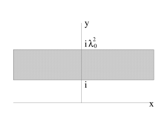
Figure 1.4: Fundamental domain of multiplication group

Now

$$d_{g}(E)=\int_{-\infty}^{\infty}\mathrm{d}x\int_{1}^{\lambda_{0}^{2}}F\left(\frac{(\lambda^{2}-1)^{2}(x^{2}+y^{2})}{\lambda^{2}y^{2}}\right)\frac{\mathrm{d}y}{y^{2}}\;.$$

Introducing a new variable $\xi=xy$ one gets

$$d_{g}(E) = \int_{1}^{\lambda_{0}^{2}}\frac{\mathrm{d}y}{y}\int_{-\infty}^{\infty}F\left((1+\xi^{2})\frac{(\lambda^{2}-1)^{2}}{\lambda^{2}}\right)\mathrm{d}\xi=$$

$$= \ln\lambda_{0}^{2}\int_{-\infty}^{\infty}F\left((1+\xi^{2})\frac{(\lambda^{2}-1)^{2}}{\lambda^{2}}\right)\mathrm{d}\xi\;.$$

After the substitution

$$u=(1+\xi^{2})\frac{(\lambda^{2}-1)^{2}}{\lambda^{2}}$$

one obtains

$$d_{g}(E)=\frac{\ln\lambda_{0}^{2}}{\sqrt{u_{0}}}\int_{u_{0}}^{\infty}\frac{F(u)}{\sqrt{u-u_{0}}}\mathrm{d}u$$

where

$$u_{0}=\frac{(\lambda^{2}-1)^{2}}{\lambda^{2}}=\lambda^{2}+\frac{1}{\lambda^{2}}-2\;.$$

The variable $u$ is connected with the distance by $\cosh d=1+u/2$ and the function $F(\cosh d)$ has the form

$$F(\cosh d)=\frac{1}{2\sqrt{2}\pi^{2}}\int_{d}^{\infty}\frac{\sin kr}{\sqrt{\cosh r-\cosh d}}\mathrm{d}r\;.$$

Introduce a variable $\tau$ connected with $r$ as $u$ is connected with $d$

$$\cosh\tau=1+\frac{r}{2}\;,\;\;\;\frac{\mathrm{d}r}{\mathrm{d}\tau}=\frac{1}{\sqrt{\tau^{2}+4\tau}}\;.$$

It gives

$$F(u)=\frac{1}{2\pi^{2}}\int_{u}^{\infty}\frac{\sin kr(\tau)}{\sqrt{(\tau-u)(\tau^{2}+4\tau)}}\mathrm{d}\tau$$

and

$$d_{g}(E)=\frac{\ln\lambda_{0}^{2}}{2\pi^{2}\sqrt{u_{0}}}f(u_{0})$$

where

$$f(w)=\int_{w}^{\infty}\frac{\mathrm{d}u}{\sqrt{u-w}}\int_{u}^{\infty}\frac{\sin kr(\tau)}{\sqrt{(\tau-u)(\tau^{2}+4\tau)}}\mathrm{d}\tau\;.$$

Changing the order of integration one obtains

$$f(w)=\int_{w}^{\infty}\frac{\sin kr(\tau)}{\sqrt{\tau^{2}+4\tau}}\mathrm{d}\tau\int_{w}^{\tau}\frac{\mathrm{d}u}{\sqrt{(u-w)(\tau-u)}}\;.$$

The last integral is a half of the residue at infinity

$$\int_{w}^{\tau}\frac{\mathrm{d}u}{\sqrt{(u-w)(\tau-u)}}=\pi$$

and

$$f(w)=\pi\int_{w}^{\infty}\frac{\sin kr(\tau)}{\sqrt{\tau^{2}+4\tau}}\mathrm{d}\tau=\pi\int_{l_{p}}^{\infty}\sin(kr)\mathrm{d}r=\frac{\pi}{k}\cos kl_{p}\;.$$

Here $l_{p}$ is the minimal value of $r$ corresponding to $u_{0}$

$$\cosh l_{p}=1+\frac{u_{0}}{2}=1+\frac{1}{2}(\lambda^{2}+\frac{1}{\lambda^{2}}-2)=\frac{1}{2}(\lambda+\frac{1}{\lambda})^{2}-1$$

or

$$2\cosh l_{p}=\lambda+\frac{1}{\lambda}\equiv\mbox{ Tr }g$$

i.e. $l_{p}$ is the length of periodic orbit associated with the matrix $g$.

Therefore

$$d_{g}(E)=\frac{\ln\lambda_{0}^{2}}{2\pi k\sqrt{\lambda+\lambda^{-1}-2}}\cos kl_{p}=\frac{l_{p}^{(0)}}{4\pi k\sinh l_{p}/2}\cos kl_{p}$$

where $l_{p}^{(0)}$ is the length of the primitive periodic orbit associated with $g_{0}$.

Combining all terms together one finds that the eigenvalues density of the Laplace–Beltrami operator automorphic with respect to a discrete group with only hyperbolic matrices has the form

$$d(E)=\frac{\mu(D)}{4\pi}\tanh\pi k+\sum_{\mbox{\scriptsize{p.p.o.}}}\frac{l_{p}}{4\pi k}\sum_{n=1}^{\infty}\frac{\cos(knl_{p})}{\sinh(nl_{p}/2)}\;.$$

The oscillating part of the density is given by the double sum. The first summation is done over all primitive periodic orbits (p.p.o.) and the second sum is performed over all repetitions of these orbits. Here $k$ is the momentum related with the energy by $E=k^{2}+1/4$.

To obtain mathematically sound formula and to avoid problems with convergence it is common to multiply both parts of the above equality by a test function $h(k)$ and to integrate over $\mathrm{d}E=2k\mathrm{d}k$. To assume the convergence the test function $h(r)$ should have the following properties

• The function $h(r)$ is a function analytical in the region $|\mbox{Im }r|\leq 1/2+\delta$ with certain $\delta>0$.

• $h(-r)=h(r)$.

• $|h(r)|\leq A(1+|r|)^{-2-\delta}$.

The left hand side of the above equation is

$$\int d(E)h(k)\mathrm{d}E=\sum_{n}\delta(E-E_{n})h(k)\mathrm{d}E=\sum_{n}h(k_{n})\;.$$

In the right hand side one obtains

$$\int h(k)\frac{\cos kl}{2\pi k}k\mathrm{d}k=\frac{1}{2\pi}\int_{-\infty}^{\infty}h(k)\mathrm{e}^{-{\rm i}kl}\mathrm{d}k\;.$$

The final formula takes the form

$$\sum_{n}h(k_{n}) = \frac{\mu(D)}{2\pi}\int_{-\infty}^{\infty}kh(k)\tanh(\pi k)\mathrm{d}k+$$ (1.29)

$$+ \sum_{\mbox{\scriptsize{p.p.o.}}}l_{p}\sum_{n=1}^{\infty}\frac{1}{2\sinh(nl_{p}/2)}g(nl_{p})$$

where $k_{n}$ is related with eigenvalue $E_{n}$ as follows

$$E_{n}=k_{n}^{2}+\frac{1}{4}$$

and $g(l)$ is the Fourier transform of $h(k)$

$$g(l)=\frac{1}{2\pi}\int_{-\infty}^{\infty}h(k)\mathrm{e}^{-{\rm i}kl}\mathrm{d}k\;.$$

This is the famous Selberg trace formula. It connects eigenvalues of the Laplace–Beltrami operator for functions automorphic with respect to a discrete group having only hyperbolic elements with classical periodic orbits.

2.9 Density of Periodic Orbits

To find the density of periodic orbits for a discrete group let us choose the test function $h(r)$ in (1.29) as

$$h(r)=\mathrm{e}^{-(r^{2}+1/4)T}\equiv\mathrm{e}^{-ET}$$

with a parameter $T>0$. Its Fourier transforms is

$$g(u)=\frac{1}{2\pi}\int_{-\infty}^{\infty}h(k)\mathrm{e}^{-{\rm i}ku}\mathrm{d}k=\frac{\mathrm{e}^{-T/4}}{2\sqrt{\pi T}}\mathrm{e}^{-u^{2}/4T}\;.$$

In the left hand side of the Selberg trace formula one obtains

$$\sum_{n}\mathrm{e}^{-E_{n}T}=1+\sum_{E_{n}>0}\mathrm{e}^{-E_{n}T}$$

where we take into account that for any discrete group there is one zero eigenvalue corresponding to a constant eigenfunction. Therefore when $T\to\infty$ the above sum tends to one

$$\sum_{n}\mathrm{e}^{-E_{n}T}\stackrel{{\scriptstyle T\to\infty}}{{\longrightarrow}}1\;.$$

One can easily check that in the right hand side of (1.29) the contribution of the smooth part of the density goes to zero at large $T$ and the contribution of periodic orbits is important only for primitive periodic orbits with $n=1$. The latter is

$$\frac{\mathrm{e}^{-T/4}}{2\sqrt{\pi T}}\sum_{\mbox{p}}l_{p}\mathrm{e}^{-l_{p}^{2}/4T-l_{p}/2}=\frac{\mathrm{e}^{-T/4}}{2\sqrt{\pi T}}\int_{0}^{\infty}l\mathrm{e}^{-l^{2}/4T-l/2}\rho(l)\mathrm{d}l$$

where $\rho(l)$ is the density of periodic orbits. Hence the Selberg trace formula states that

$$\lim_{T\to\infty}\frac{\mathrm{e}^{-T/4}}{2\sqrt{\pi T}}\int_{0}^{\infty}l\mathrm{e}^{-l^{2}/4T-l/2}\rho(l)\mathrm{d}l=1\;.$$

Assume that $\rho(l)=b\mathrm{e}^{al}/l$ with certain constants $a$ and $b$. Then from the above limit it follows that $a=b=1$ which demonstrates that the density of periodic orbits for a discrete group increases exponentially with the length

$$\rho(l)=\frac{\mathrm{e}^{l}}{l}\;.$$

2.10 Selberg Zeta Function

Amongst many applications of the Selberg trace formula let us consider the construction of the Selberg zeta function.

Choose as test function $h(k)$ the function

$$h(k)=\frac{1}{k^{2}+\alpha^{2}}-\frac{1}{k^{2}+\beta^{2}}\;.$$

Its Fourier transform is

$$g(l)=\frac{1}{2\alpha}\mathrm{e}^{-\alpha|l|}-\frac{1}{2\beta}\mathrm{e}^{-\beta|l|}\;.$$

The Selberg trace formula gives

$$\sum_{n}\left(\frac{1}{k_{n}^{2}+\alpha^{2}}-\frac{1}{k_{n}^{2}+\beta^{2}}\right)=$$

$$=\frac{\mu(D)}{2\pi}\int_{-\infty}^{\infty}k\tanh\pi k\left(\frac{1}{k^{2}+\alpha^{2}}-\frac{1}{k^{2}+\beta^{2}}\right)\mathrm{d}k+$$

$$+\sum_{\mbox{\scriptsize{p.p.o.}}}\sum_{n=1}^{\infty}\frac{l_{p}}{2\sinh nl_{p}/2}\left(\frac{\mathrm{e}^{-\alpha l_{p}}}{2\alpha}-\frac{\mathrm{e}^{-\beta l_{p}}}{2\beta}\right)\;.$$

The Selberg zeta function is defined as the following formal product

$$Z(s)=\prod_{\mbox{\scriptsize{p.p.o}}}\prod_{m=0}^{\infty}(1-\mathrm{e}^{-l_{p}(s+m)})\;.$$ (1.30)

One has

$$\frac{1}{Z}\frac{dZ}{ds} = \sum_{\mbox{\scriptsize{p.p.o.}}}\sum_{m=0}^{\infty}\frac{l_{p}\mathrm{e}^{-l_{p}(s+m)}}{1-\mathrm{e}^{-l_{p}(s+m)}}=\sum_{\mbox{\scriptsize{p.p.o.}}}l_{p}\sum_{n=1}^{\infty}\sum_{m=0}^{\infty}\mathrm{e}^{-l_{p}(s+m)n}=$$

$$= \sum_{\mbox{p.p.o.}}l_{p}\sum_{n=1}^{\infty}\frac{\mathrm{e}^{-l_{p}ns}}{1-\mathrm{e}^{-l_{p}n}}=\sum_{\mbox{\scriptsize{p.p.o.}}}l_{p}\sum_{n=1}^{\infty}\frac{1}{2\sinh nl_{p}/2}\mathrm{e}^{-l_{p}n(s-1/2)}\;.$$

Choose $\alpha=s-1/2$ and $\beta=s^{\prime}-1/2$ then

$$\sum_{n}\left(\frac{1}{k_{n}^{2}+(s-1/2)^{2}}-\frac{1}{k_{n}^{2}+(s^{\prime}-1/2)^{2}}\right)=$$

$$=\frac{\mu(D)}{4\pi}\int_{-\infty}^{\infty}k\tanh\pi k\left(\frac{1}{k^{2}+(s-1/2)^{2}}-\frac{1}{k^{2}+(s^{\prime}-1/2)^{2}}\right)\mathrm{d}k+$$

$$+\frac{1}{2s-1}\frac{Z(s)^{\prime}}{Z(s)}-\frac{1}{2s^{\prime}-1}\frac{Z(s^{\prime})^{\prime}}{Z(s^{\prime})}\;.$$

The integral in the right hand side can be computed by the residues

$$\int_{-\infty}^{\infty}k\tanh\pi k\left(\frac{1}{k^{2}+(s-1/2)^{2}}-\frac{1}{k^{2}+(s-1/2)^{2}}\right)\mathrm{d}k=f(s)-f(s^{\prime})$$

where $f(s)$ is the sum over residues from one pole $k=i(s-1/2)$ and from poles $k_{n}=i(n+1/2)$ of $\tanh\pi k$

$$f(s)=2\pi{\rm i}\left[\frac{1}{2}\tanh[{\rm i}\pi(s-1/2)]+\frac{{\rm i}}{\pi}\sum_{n=0}^{\infty}\frac{n+1/2}{(s-1/2)^{2}-(n+1/2)^{2}}\right]=$$

$$=\pi\cot\pi s-\sum_{n=1}^{\infty}\frac{1}{s-n}+\sum_{n=1}^{\infty}\frac{1}{s+n}\;.$$

But

$$\pi\cot\pi s=\sum_{n=1}^{\infty}\frac{1}{s-n}+\sum_{n=1}^{\infty}\frac{1}{s+n}\;,$$

therefore

$$f(s)=2\sum_{n=1}^{\infty}\frac{1}{s+n}\;.$$

Using these relations one gets the identity valid for all values of $s$ and $s^{\prime}$

$$\frac{1}{2s-1}\frac{Z^{\prime}(s)}{Z(s)} = \frac{1}{2s^{\prime}-1}\frac{Z^{\prime}(s^{\prime})}{Z(s^{\prime})}-\frac{\mu(D)}{2\pi}\sum_{n=0}^{\infty}\left(\frac{1}{s+n}-\frac{1}{s^{\prime}+n}\right)+$$ (1.31)

$$+ \sum_{n}\left(\frac{1}{k_{n}^{2}+(s-1/2)^{2}}-\frac{1}{k_{n}^{2}+(s^{\prime}-1/2)^{2}}\right)\;.$$

The right hand side of this identity has poles at $s=1/2+{\rm i}k_{n}$ and $s=-n$. The same poles have to be present in the left hand side. If

$$\frac{Z^{\prime}(s)}{Z(s)}\to\frac{\nu_{k}}{s-s_{k}}$$

then

$$Z(s)\to(s-s_{k})^{\nu_{k}}\;\;\;\mbox{when }s\to s_{k}\;.$$

When $\nu_{k}>0$ (resp. $\nu_{k}<0$) point $s_{k}$ is a zero (resp. a pole) of the Selberg zeta function $Z(s)$.

2.11 Zeros of the Selberg Zeta Function

Combining all poles one concludes that the Selberg zeta function for a group with only hyperbolic elements have two different sets of zero. The first consists of non-trivial zeros

$$s=1/2\pm{\rm i}k_{n},$$

coming from eigenvalues of the Laplace–Beltrami operator for automorphic functions. The second set includes a zero from $E=0$ eigenvalue and zeros from the smooth term. These zeros are called trivial zeros and they are located at points

$$s=-m\;\;(m=1,2,\ldots$$

with multiplicity $\nu_{m}=(2m+1)\mu(D)/2\pi$, at point $s=0$ with multiplicity $\nu_{0}=\mu(D)/2\pi$ and a single zero at $s=1$. These multiplicities are integers because the area of a compact fundamental domain $\mu(D)=4\pi(g-1)$ where $g$ is the genus of the surface.

The structure of these zeros is presented schematically at Fig. 1.5.

Figure 1.5: Zeros of the Selberg zeta function

2.12 Functional Equation

The infinite product defining the Selberg zeta function (1.30) converges only when Re $s>1/2$. Nevertheless the Selberg zeta function can be analytically continued to the whole complex plane $s$ with the aid of (1.31).

Put $s^{\prime}=1-s$ in (1.31). The sum over eigenvalues cancels and $f(s)-f(1-s)=2\pi\cot\pi s$. Therefore

$$\frac{1}{2s-1}\left(\frac{Z^{\prime}(s)}{Z(s)}+\frac{Z^{\prime}(1-s)}{Z(1-s)}\right)=-\frac{\mu(D)}{2}\cot\pi s$$

which is equivalent to the following relation (called functional equation)

$$Z(s)=\varphi(s)Z(1-s)$$ (1.32)

where

$$\frac{\varphi^{\prime}(s)}{\varphi(s)}=-\mu(D)(s-\frac{1}{2})\cot\pi s$$

and $\varphi(1/2)=1$.

Explicitly

$$\varphi(s)=\exp\left(\mu(D)\int_{0}^{s-1/2}u\tan\pi u\mathrm{d}u\right)\;.$$

Therefore if one knows the Selberg zeta function when Re $s>1$ (1.32) gives its continuation to the mirror region Re $s<0$.

3 Trace Formulas for Integrable Dynamical Systems

A $f$-dimensional system is called integrable if its classical Hamiltonian can be written as a function of action variables only

$$H(\vec{I})=H(I_{1},\ldots,I_{f})\;.$$

In this representation the classical equations of motion take especially simple form

$$\dot{\vec{I}}=-\frac{\partial H}{\partial\vec{\varphi}}=0\;,\;\;\dot{\vec{\varphi}}=\frac{\partial H}{\partial\vec{I}}=\vec{\omega}\;.$$

The semiclassical quantization consists of fixing the values of the action variables

$$I_{j}=\hbar(n_{j}+\frac{\mu_{j}}{4})$$

where $n_{j}$ are integers and $\mu_{j}$ are called the Maslov indices.

In this approximation eigenvalues of energy of the system are a function of these integers

$$E(\vec{n})=H\left(\hbar(n_{1}+\frac{\mu_{1}}{4}),\ldots,\hbar(n_{f}+\frac{\mu_{f}}{4})\right)\;.$$

The eigenvalue density is the sum over all integers $n_{j}$

$$d(E)=\sum_{\vec{n}}\delta(E-H(\hbar(\vec{n}+\frac{1}{4}\vec{\mu}))\;.$$

Using the Poisson summation formula (1.5) one transforms this expression as follows

$$d(E) = \sum_{\vec{N}}\int e^{2\pi i\vec{N}\vec{n}}\delta(E-H(\hbar(\vec{n}+\frac{1}{4}\vec{\mu}))\mathrm{d}\vec{n}=$$ (1.33)

$$= \frac{1}{\hbar^{f}}\sum_{\vec{N}}\mathrm{e}^{-{\rm i}\pi\vec{N}\vec{\mu}/2}\int\mathrm{e}^{2\pi i\vec{N}\vec{I}/\hbar}\int\delta(E-H(\vec{I}\,))\mathrm{d}\vec{I}$$

where the summation is taken over $f$ integers $N_{j}$.

3.1 Smooth Part of the Density

The term with $\vec{N}=0$ in (1.33) corresponds to the smooth part of the density

$$\bar{d}(E)=\frac{1}{\hbar^{f}}\int\delta(E-H(\vec{I}\,))\mathrm{d}\vec{I}\;.$$

As $\mathrm{d}\vec{I}\mathrm{d}\vec{\varphi}$ is the canonical invariant, $\mathrm{d}\vec{I}\mathrm{d}\vec{\varphi}=\mathrm{d}\vec{p}\mathrm{d}\vec{q}$ where $\vec{p}$ and $\vec{q}$ are the momenta and coordinates and, because $\int\mathrm{d}\vec{\varphi}=(2\pi)^{f}$, the formula for the smooth part of the level density can be rewritten in the Thomas-Fermi form

$$\bar{d}(E)=\int\delta(E-H(\vec{p},\vec{q}\,))\frac{\mathrm{d}\vec{p}\mathrm{d}\vec{q}}{(2\pi\hbar)^{f}}\;.$$ (1.34)

The usual interpretation of this formula is that each quantum state occupies $(2\pi\hbar)^{f}$ volume on the constant energy surface. For general systems (1.34) represents the leading term of the expansion of the smooth part of the level density when $\hbar\to 0$. Other terms can be found e.g. in BaltesHill . See also BerryHowls for the resummation of such series for certain models.

3.2 Oscillating Part of the Density

In the semiclassical approximation $\hbar\to 0$ terms with $\vec{N}\neq 0$ in (1.33) can be calculated by the saddle point method. Our derivation differs slightly from the one given in TaborBerry . First it is convenient to represent $\delta$-function as follows

$$\delta(x)=\frac{1}{2\pi\hbar}\int_{-\infty}^{\infty}\mathrm{e}^{{\rm i}\alpha x/\hbar}\mathrm{d}\alpha\;.$$

Then

$$d^{(osc)}(E)=\frac{1}{2\pi\hbar^{f+1}}\sum_{\vec{N}}\mathrm{e}^{-{\rm i}\pi\vec{N}\vec{\mu}/2}\int_{-\infty}^{\infty}\mathrm{d}\alpha\int\mathrm{e}^{{\rm i}S(\vec{I},\alpha)/\hbar}\mathrm{d}\vec{I}$$

where the effective action, $S(\vec{I},\alpha)$, is

$$S(\vec{I},\alpha)=2\pi\vec{N}\vec{I}+\alpha(E-H(\vec{I}))\;.$$

The integration over $\vec{I}$ and $\alpha$ can be performed by the saddle point method. The saddle point values, $\vec{I}_{sp}$ and $\alpha_{sp}$, are determined from equations

$$\frac{\partial S}{\partial\alpha}=E-H(\vec{I}_{sp})=0\;,\;\;\;\frac{\partial S}{\partial\vec{I}}=2\pi\vec{N}-\alpha_{sp}\vec{\omega}_{sp}=0\;.$$

The first equation shows that in the leading approximation $\vec{I}_{sp}$ belongs to the constant energy surface and the second equation selects special values of $\vec{I}_{sp}$ for which frequencies $\omega_{j}$ are commensurable

$$\vec{\omega}_{sp}=\frac{2\pi}{\alpha_{sp}}\vec{N}\;.$$

Together the saddle point conditions demonstrate that in the limit $\hbar\to 0$ the dominant contribution to the term with fixed integer vector $\vec{N}$ comes from the classical periodic orbit with period

$$T_{p}=\alpha_{s.p}$$

and the saddle point action coincides with the classical action along this trajectory

$$S_{sp}=2\pi\vec{N}\vec{I}_{sp}\;.$$

To compute remaining integrals it is necessary to expand the full action up to quadratic terms on deviations from the saddle point values. One has

$$S(\vec{I}_{sp}+\delta\vec{I},\alpha_{s.p}+\delta\alpha)=S_{sp}+\frac{T_{p}}{2}(\delta I_{i}H_{ij}\delta I_{j})-\delta\alpha(\omega_{j}\delta I_{j})$$

where the summation over repeating indexes is assumed. $H_{ij}$ is the matrix of the second derivatives of the Hamiltonian computed at the saddle point

$$H_{ij}\equiv\frac{\partial^{2}H}{\partial I_{i}\partial I_{j}}\left|{}_{\vec{I}=\vec{I}_{sp}}\right.\;.$$

The following steps are straightforward

$$\int\mathrm{d}\delta\vec{I}\mathrm{d}\delta\alpha\exp\left(\frac{{\rm i}}{\hbar}S(\vec{I},\alpha)\right)=$$

$$= \mathrm{e}^{{\rm i}S_{sp}/\hbar}\int\mathrm{d}\delta\alpha\int\mathrm{d}\delta\vec{I}\exp\left(\frac{{\rm i}}{2\hbar}T_{p}(\delta I_{i}H_{ij}\delta I_{j})-\frac{\delta\alpha}{\hbar}(\omega_{j}\delta I_{j})\right)=$$

$$= \left(\frac{2\pi\hbar}{T_{p}}\right)^{f/2}\frac{\mathrm{e}^{{\rm i}S_{sp}/\hbar}}{\sqrt{|\det H_{ij}|}}\int\delta\alpha\exp\left(-\frac{{\rm i}}{2\hbar T_{p}}(\delta\alpha)^{2}(\omega_{i}H_{ij}^{-1}\omega_{j})+\frac{{\rm i}}{4}\pi\beta^{\prime}\right)=$$

$$= \left(\frac{2\pi\hbar}{T_{p}}\right)^{f/2}\frac{\sqrt{2\pi\hbar T_{p}}}{\sqrt{|\det H_{ij}|(\omega_{k}H_{kl}^{-1}\omega_{l})}}\exp\left(\frac{{\rm i}}{\hbar}S_{sp}+\frac{{\rm i}}{4}\pi\beta\right)=$$

$$= \frac{(2\pi)^{(f-1)/2}\hbar^{(f+1)/2}}{T_{p}^{(f-3)/2}|(N_{i}Q_{ij}N_{j})|^{1/2}}\exp\left(\frac{{\rm i}}{\hbar}S_{sp}+\frac{{\rm i}}{4}\pi\beta\right)$$

where $Q_{ij}=H_{ij}^{-1}\det H$ called the co-matrix of $H_{ij}$ is the determinant obtained from $H_{ij}$ by omitting the $i$-th row and the $j$-th column. The phase $\beta$ is the signature of $H_{ij}$ minus the sign of $(\omega H^{-1}\omega)$.

The final expression for the oscillating part of the level density of an integrable system with a Hamiltonian $H(\vec{I})$ is

$$d^{(osc)}(E)=\sum_{\vec{N}}P_{\vec{N}}\exp\left({\rm i}\frac{S_{p}}{\hbar}-{\rm i}\frac{\pi}{4}\vec{N}\vec{\mu}+{\rm i}\frac{\pi}{4}\beta\right)$$

where $S_{p}=2\pi\vec{N}\vec{I}$ is the action over a classical periodic orbit with fixed winding numbers and

$$P_{\vec{N}}=\left(\frac{2\pi}{\hbar T_{p}}\right)^{(f-3)/2}\frac{1}{\hbar^{2}|(N_{i}Q_{ij}N_{j})|^{1/2}}\;.$$

The summation over integer vectors $\vec{N}$ is equivalent to the summation over all classical periodic orbit families of the system.

4 Trace Formula for Chaotic Systems

To compute the eigenvalue density for a chaotic system one has to start with general expression (1.17)

$$d(E)=-\frac{1}{\pi}\int\mbox{Im }G_{E}(\vec{x},\vec{x})\mathrm{d}\vec{x}$$

which relates the quantum density with the Green function of the system, $G_{E}(\vec{x},\vec{y})$, obeying the Schroedinger equation with a $\delta$-function term in the right hand side

$$(E-\hat{H})G_{E}(\vec{x},\vec{y})=\delta(\vec{x}-\vec{y})\;.$$

For concreteness let us consider the usual case

$$\hat{H}=-\hbar^{2}\varDelta+V(\vec{x})\;.$$

The exact Green function can be computed exactly only in very limited cases. For generic systems the best which can be achieved is the calculation of the Green function in the semiclassical limit $\hbar\to 0$.

4.1 Semiclassical Green Function

Let us try to obey the Schroedinger equation in the following form (see Gutzwiller )

$$G_{E}(\vec{x},\vec{y})=A(\vec{x},\vec{y})\mathrm{e}^{{\rm i}S(\vec{x},\vec{y})/\hbar}$$ (1.35)

where the prefactor $A(\vec{x},\vec{y})$ can be expanded into a power series of $\hbar$.

Separating the real and imaginary parts of the Schroedinger equation one gets two equations

$$\left(E-(\nabla S)^{2}-V(\vec{x})\right)+\hbar^{2}\varDelta A=0$$

and

$$2\nabla S\nabla A+\varDelta SA=0\;.$$

In the leading order in $\hbar$ the first equation reduces to the Hamilton-Jacobi equation for the classical action $S(\vec{x},\vec{y})$

$$E=(\nabla S)^{2}+V(\vec{x})\;.$$

It is well known that the solution of this equation can be obtained in the following way.

Find the solution of the usual classical equations of motion

$$\ddot{\vec{x}}=-\frac{\partial V}{\partial\vec{x}}$$

with energy $E$ which starts at a fixed point $\vec{y}$ and ends at a point $\vec{x}$. Then

$$S(\vec{x},\vec{y})=\int_{\vec{y}}^{\vec{x}}\vec{p}d\vec{x}$$

where $\vec{p}$ is the momentum and the integral is taken over this trajectory.

Instead of proving this fact we illustrate it on an example of the free motion. The free motion equations $\ddot{\vec{x}}=0$ have a general solution

$$\vec{x}=\vec{k}t+\vec{y}$$

with a fixed vector $\vec{k}$. One has

$$\vec{k}=\frac{\vec{x}-\vec{y}}{t}$$

and the conservation of energy $|\vec{k}|^{2}=E$ determines the time of motion

$$t=\frac{|\vec{x}-\vec{y}|}{\sqrt{E}}\;.$$

Therefore

$$S(\vec{x},\vec{y})=\sqrt{E}|\vec{x}-\vec{y}|$$

which, evidently, is the solution of the free Hamilton–Jacobi equation.

The next order equation

$$2\nabla S\nabla A+\varDelta SA=0$$

is equivalent to the conservation of current. Indeed, for the semiclassical wave function (1.35)

$$\vec{J}=\frac{1}{2{\rm i}}(\Psi^{*}\nabla\Psi-\Psi\nabla\Psi^{*})=A^{2}\nabla S$$

and

$$\nabla\vec{J}=A(2\nabla A\nabla S+A\varDelta S)=0\;.$$

The solution of the above transport equation has the form

$$A(\vec{x},\vec{y})=\frac{\pi}{(2\pi\hbar)^{(f+1)/2}}\left|\frac{1}{k_{i}k_{f}}\det\left(-\frac{\partial^{2}S}{\partial t_{i\bot}\partial t_{f\bot}}\right)\right|^{1/2}$$

where $t_{i\bot}$ and $t_{f\bot}$ are coordinates perpendicular to the trajectory in the initial, $\vec{y}$, and final, $\vec{x}$, points respectively and $k_{i}$, $k_{f}$ are the initial and final momenta. The derivation of this formula can be found e.g. in Gutzwiller . The overall prefactor in this formula can be fixed by comparing with the asymptotics of the free Green function (1.14) at large distances.

The final formula for the semiclassical Green function takes the form

$$G_{E}(\vec{x},\vec{y}) = \sum_{\begin{array}[]{c}\mbox{\scriptsize{classical}}\\ \mbox{\scriptsize{trajectories}}\end{array}}\frac{\pi}{(2\pi\hbar)^{(f+1)/2}}\left|\frac{1}{k_{i}k_{f}}\det\left(-\frac{\partial^{2}S}{\partial t_{i\bot}\partial t_{f\bot}}\right)\right|^{1/2}\times$$

$$\times \exp\left(\frac{{\rm i}}{\hbar}S_{cl}(\vec{x},\vec{y})-\frac{{\rm i}}{4}\pi\mu\right)$$

where the sum is taken over all classical trajectories with energy $E$ which connect points $\vec{y}$ and $\vec{x}$. $\mu$ is the Maslov index which, roughly speaking, counts the number of points along the trajectory where semiclassical approximation cannot be applied.

4.2 Gutzwiller Trace Formula

The knowledge of the Green function permits the calculation of the density of eigenstates by the usual formula (1.17)

$$d(E)=-\frac{1}{\pi}\int\mbox{ Im }G_{E}(\vec{x},\vec{x})\mathrm{d}\vec{x}\;.$$

The Green function $G_{E}(\vec{x},\vec{y})$ at points $\vec{x}$ and $\vec{y}$ very close to each other has two different contributions (see Fig. 1.6).

Figure 1.6: Small and large action contributions to the Green function for nearby points

The first comes from very short trajectories where semiclassical approximation cannot, in general, be applied. The second is related with long trajectories. The first contribution can be computed by using the Thomas–Fermi (local) approximation for the Green function. In this approximation one uses the local formula (cf. (1.16))

$$G_{E}(\vec{x},\vec{y})\stackrel{{\scriptstyle\vec{y}\to\vec{x}}}{{\longrightarrow}}\int\frac{\mathrm{d}\vec{p}}{(2\pi\hbar)^{f}}\frac{\mathrm{e}^{i\vec{p}(\vec{x}-\vec{y})/\hbar}}{(E-H(\vec{p},\vec{x})+i\epsilon)}\;.$$

Therefore

$$\mbox{ Im }G_{E}(\vec{x},\vec{x})=-\pi\int\frac{\mathrm{d}\vec{p}}{(2\pi\hbar)^{f}}\delta\left(E-H(\vec{p},\vec{x})\right)$$

and the smooth part of the level density in the leading approximation equals the phase-space volume of the constant energy surface divided by $(2\pi\hbar)^{f}$

$$\bar{d}(E)=\int\frac{\mathrm{d}\vec{p}\mathrm{d}\vec{x}}{(2\pi\hbar)^{f}}\delta\left(E-H(\vec{p},\vec{x})\right)\;.$$

The contributions from long classical trajectories with finite actions corresponds to the oscillating part of the density and can be calculated using the semiclassical approximation of the Green function (1.35).

One has

$$d^{(osc)}(E)=-\frac{1}{\pi}\mbox{ Im }\sum_{\begin{array}[]{c}\mbox{\scriptsize{classical}}\\ \mbox{\scriptsize{trajectories}}\end{array}}\int A(\vec{x},\vec{x})\mathrm{e}^{{\rm i}S(\vec{x},\vec{x})/\hbar}\mathrm{d}\vec{x}\;.$$

When $\hbar\to 0$ the integration can be performed in the saddle point approximation. The saddles are solutions of the equation

$$\left[\frac{\partial S(\vec{x},\vec{y})}{\partial\vec{x}}+\frac{\partial S(\vec{x},\vec{y})}{\partial\vec{y}}\right]_{\vec{y}=\vec{x}}=0\;.$$

But

$$\frac{\partial S(\vec{x},\vec{y})}{\partial\vec{x}}=\vec{k}_{f}\;,\;\;\;\frac{\partial S(\vec{x},\vec{y})}{\partial\vec{y}}=-\vec{k}_{i}$$

where $\vec{k}_{f}$ and $\vec{k}_{i}$ are the momenta in the final and initial points respectively.

Hence the saddle point equations select special classical orbits which start and end in the same point with the same momentum. It means that the saddles are classical periodic orbits of the system and

$$S_{sp}=S_{p}\;.$$

To calculate the integral around one particular periodic orbit it is convenient to split the integration over the whole space to one integration along the orbit and $(f-1)$ integrations in directions perpendicular to the orbit. For simplicity we consider the two-dimensional case.

The change of the action when a point is at the distance $y$ from the periodic orbit is

$$\delta S=\frac{1}{2}y^{2}\frac{\partial^{2}S(y,y)}{\partial y^{2}}|_{y=0}$$

where $S(y,y)$ is the classical action for a classical orbit in a vicinity of the periodic orbit (see Fig. 1.7).

Figure 1.7: A periodic orbit and a closed classical orbit in its vicinity

To compute such derivatives it is useful to use the monodromy matrix, $m_{ij}$, which relates initial and final coordinates and momenta in a vicinity of periodic orbit in the linear approximation

$$\left(\begin{array}[]{c}\delta y_{f}\\ \delta p_{f}\end{array}\right)=\left(\begin{array}[]{cc}m_{11}&m_{12}\\ m_{21}&m_{22}\end{array}\right)\left(\begin{array}[]{c}\delta y_{i}\\ \delta p_{i}\end{array}\right)\;.$$

As the classical motion preserves the canonical invariant $\mathrm{d}p\mathrm{d}q$ it follows that $\det M=1$.

One has

$$\delta y_{f} = m_{11}\delta y_{i}+m_{12}\delta p_{i}\;,$$

$$\delta p_{f} = m_{21}\delta y_{i}+m_{22}\delta p_{i}\;.$$

But

$$p_{i}=-\frac{\partial S}{\partial y_{i}}\;,\;\;\;p_{f}=\frac{\partial S}{\partial y_{f}}\;.$$

Therefore

$$\delta p_{i}=-\frac{\partial^{2}S}{\partial y_{i}^{2}}\delta y_{i}-\frac{\partial^{2}S}{\partial y_{i}\partial y_{f}}\delta y_{f}\;,\;\;\delta p_{f}=\frac{\partial^{2}S}{\partial y_{i}\partial y_{f}}\delta y_{i}+\frac{\partial^{2}S}{\partial y_{f}^{2}}\delta y_{f}\;.$$

From comparison of these two expression one obtains the expressions of the second derivatives of the action through monodromy matrix elements

$$\frac{\partial^{2}S}{\partial y_{i}\partial y_{f}}=-\frac{1}{m_{12}}\;,\;\;\frac{\partial^{2}S}{\partial y_{i}^{2}}=\frac{m_{11}}{m_{12}}\;,\;\;\frac{\partial^{2}S}{\partial y_{f}^{2}}=\frac{m_{22}}{m_{12}}\;.$$

Substituting these expressions to the contribution to the trace formula from one periodic orbit one gets (in two dimensions)

$$d^{(osc)}_{p}(E)=\frac{1}{{\rm i}(2\pi{\rm i}\hbar)^{3/2}}\int|m_{12}|^{-1/2}\exp(\frac{{\rm i}}{\hbar}S_{p}+{\rm i}\frac{m_{11}+m_{22}-2}{2\hbar\;m_{12}}y^{2})\mathrm{d}y\frac{\mathrm{d}x}{k(x)}$$

where $x$ and $y$ are respectively coordinates parallel and perpendicular to the trajectory.

Computing the resulting integrals one obtains

$$d^{(osc)}_{p}(E)=\frac{T_{p}}{\pi\hbar}\frac{\mathrm{e}^{{\rm i}S_{p}/\hbar-{\rm i}\pi\mu_{p}/2}}{\sqrt{|m_{11}+m_{22}-2|}}$$

where $T_{p}=\int\mathrm{d}x/k(x)$ is the geometrical period of the trajectory.

Finally the Gutzwiller trace formula takes the form (valid in arbitrary dimensions)

$$d^{(osc)}(E)=\sum_{\begin{array}[]{c}\mbox{\scriptsize{primitive}}\\ \mbox{\scriptsize{periodic}}\\ \mbox{\scriptsize{orbits}}\end{array}}\frac{T_{p}}{\pi\hbar}\sum_{n=1}^{\infty}\frac{1}{|\det(M_{p}^{n}-1)|^{1/2}}\cos\left[n(\frac{S_{p}}{\hbar}-\frac{\pi}{2}\mu_{p})\right]\;.$$

In the derivation of this formula we assumed that all periodic orbits are unstable and $M_{p}$ is the monodromy matrix for a primitive periodic orbit.

5 Riemann Zeta Function

The trace-like formulas exist not only for dynamical systems but also for the Riemann zeta function (and others number-theoretical zeta functions as well).

The Riemann zeta function is a function of complex variable $s$ defined as follows

$$\zeta(s)=\sum_{n=1}^{\infty}\frac{1}{n^{s}}=\prod_{p}(1-p^{-s})^{-1}$$ (1.37)

where the product is taken over prime numbers. The second equality (called the Euler product) is a consequence of the unique factorization of integers into a product of prime numbers.

This function converges only when Re$s>1$ but can analytically be continued in the whole complex $s$-plane.

5.1 Functional Equation

The possibility of this continuation is connected with the fact that the Riemann zeta function satisfies the important functional equation

$$\zeta(s)=\varphi(s)\zeta(1-s)$$ (1.38)

where

$$\varphi(s)=2^{s}\pi^{s-1}\sin\left(\frac{\pi s}{2}\right)\Gamma(1-s)\;.$$ (1.39)

We present one of numerous method of proving this relation (see e.g. Titchmarsh ).

When Re $s>0$ one has the equality

$$\int_{0}^{\infty}x^{s/2-1}\mathrm{e}^{-\pi n^{2}x}\mathrm{d}x=\frac{\Gamma(s/2)}{n^{s}\pi^{s/2}}$$

where $\Gamma(x)$ is the Gamma function (see e.g. Bateman , Vol. 1, Sect. 1). Therefore if Re $s>1$

$$\frac{\Gamma(s/2)\zeta(s)}{\pi^{s/2}}=\int_{0}^{\infty}x^{s/2-1}\Psi(x)\mathrm{d}x$$

where $\Psi(x)$ is given by the following series

$$\Psi(x)=\sum_{n=1}^{\infty}\mathrm{e}^{-\pi n^{2}x}\;.$$

Using the Poisson summation formula (1.5) one obtains

$$\sum_{n=-\infty}^{\infty}\mathrm{e}^{-\pi n^{2}x}=\frac{1}{\sqrt{x}}\sum_{n=-\infty}^{\infty}\mathrm{e}^{-\pi n^{2}/x}$$

which leads to the identity

$$2\Psi(x)+1=\frac{1}{\sqrt{x}}\left(2\Psi(\frac{1}{x})+1\right)\;.$$

Hence

$$\xi(s) \equiv \pi^{-s/2}\Gamma(\frac{1}{2}s)\zeta(s)=\int_{0}^{1}x^{s/2}\Psi(x)\mathrm{d}x+\int_{1}^{\infty}x^{s/2}\Psi(x)\mathrm{d}x=$$

$$= \int_{0}^{1}x^{s/2}\left(\frac{1}{\sqrt{x}}\Psi(\frac{1}{x})+\frac{1}{2\sqrt{x}}-\frac{1}{2}\right)\mathrm{d}x+\int_{1}^{\infty}x^{s/2}\Psi(x)\mathrm{d}x=$$

$$= \frac{1}{s-1}-\frac{1}{s}+\int_{0}^{1}x^{s/2-3/2}\Psi(\frac{1}{x})\mathrm{d}x+\int_{1}^{\infty}x^{s/2}\Psi(x)\mathrm{d}x=$$

$$= \frac{1}{s(s-1)}+\int_{1}^{\infty}\left(x^{-s/2-1/2}+x^{s/2-1}\right)\Psi(x)\mathrm{d}x\;.$$

The last integral is convergent for all values of $s$ and gives the analytical continuation of the Riemann zeta function to the whole complex $s$-plane, the only singularity being the pole at $s=1$ with unit residue

$$\zeta(s)\stackrel{{\scriptstyle s\to 1}}{{\longrightarrow}}\frac{1}{s-1}\;.$$

(The pole at $s=0$ is canceled by the pole of $\Gamma(s/2)$ giving $\zeta(0)=-1/2$.)

One of important consequences of the above formula of analytical continuation is that it does not change under the substitution $s\to 1-s$. Therefore for all values of $s$

$$\xi(s)=\xi(1-s)$$

or

$$\zeta(s)=\varphi(s)\zeta(1-s)$$

where

$$\varphi(s)=\pi^{s-1/2}\frac{\Gamma(1/2-s/2)}{\Gamma(s/2)}$$ (1.40)

By standard formulas (see e.g. Bateman , Vol. 1, 1.2.5, 1.2.15)

$$\Gamma(x)\Gamma(1-x)=\frac{\pi}{\sin\pi x}\;,\;\;\;\Gamma(2x)=2^{2x-1}\pi^{-1/2}\Gamma(x)\Gamma(x+\frac{1}{2})$$

the last expression can be transformed to (1.39) which proves the functional equation (1.38).

From the functional equation (1.38) is follows that $\zeta(s)$ has ’trivial’ zeros at negative even integers (except zero) $s=-2,-4,\ldots$ which appear from $\sin(\pi s/2)$ in (1.39). All other non-trivial zeros, $\zeta(s_{n})=0$, are situated in the so-called critical strip $0<\mbox{ Re }s<1$. If one denotes these zeros as $s_{n}=1/2+{\rm i}\gamma_{n}$ then functional equation together with the fact that $\zeta(s)^{*}=\zeta(s^{*})$ state that in general there exit 4 sets of zeros: $\gamma_{n}\;,\;-\gamma_{n}\;,\;\gamma_{n}^{*}\;,\;-\gamma_{n}^{*}$.

According to the famous Riemann conjecture (see e.g. Titchmarsh ) all nontrivial zeros of $\zeta(s)$ lie at the symmetry line Re $s=1/2$ or $\gamma_{n}$ are all real quantities. Numerical calculations confirms this conjecture for exceptionally large number of zeros (see e.g. OdlyzkoPaper and the web site of Odlyzko Web ) but a mathematical proof is still absent.

5.2 Trace Formula for the Riemann Zeros

Let us fix a test function $h(r)$ exactly as it was done for the Selberg trace formula in Sect. 2.8 i.e.

• $h(r)$ is a function analytical in the region $|\mbox{Im }r|$ $\leq 1/2+\delta$,

• $h(-r)=h(r)$,

• $|h(r)|\leq A(1+|r|)^{-2-\delta}$.

Denote as in that Section

$$g(u)=\frac{1}{2\pi}\int_{-\infty}^{+\infty}h(r)\mathrm{e}^{-iru}\mathrm{d}r$$

and define

$$H(s)=\int_{-\infty}^{+\infty}g(u)\mathrm{e}^{(s-1/2)u}\mathrm{d}u\;.$$

Now let us compute the integral

$$\frac{1}{2\pi{\rm i}}\oint\mathrm{d}sH(s)\frac{\zeta^{\prime}(s)}{\zeta(s)}$$

where the contour of integration is taken over the rectangle $-\eta\leq\mbox{ Re }s\leq 1+\eta$ and $-T\leq\mbox{ Im }s\leq T$ with $0<\eta<\delta$ and $T\to+\infty$. Inside this rectangle there are poles of $\zeta^{\prime}(s)/\zeta(s)$ coming from non-trivial zeros of the Riemann zeta function, $s_{n}=1/2+{\rm i}\gamma_{n}$, and the one from the pole of $\zeta(s)$ at $s=1$. The total contribution from these poles is

$$\sum_{n}h(\gamma_{n})-h(-\frac{{\rm i}}{2})\;.$$

One can check that the limit $T\to\infty$ exists and, consequently, one has the identity

$$\sum_{n}h(\gamma_{n})-h(-\frac{{\rm i}}{2})=\frac{1}{2\pi{\rm i}}\int_{1+\eta-{\rm i}\infty}^{1+\eta+{\rm i}\infty}\mathrm{d}sH(s)\frac{\zeta^{\prime}(s)}{\zeta(s)}-\frac{1}{2\pi{\rm i}}\int_{-\eta-{\rm i}\infty}^{-\eta+{\rm i}\infty}\mathrm{d}sH(s)\frac{\zeta^{\prime}(s)}{\zeta(s)}\;.$$

Let us substitute in the second integral the functional equation (1.38) with $\varphi(s)$ from (1.40). One has

$$\frac{\zeta^{\prime}(s)}{\zeta(s)}=\ln\pi-\frac{\zeta^{\prime}(1-s)}{\zeta(1-s)}-\frac{1}{2}\left[\frac{\Gamma^{\prime}}{\Gamma}\left(\frac{s}{2}\right)+\frac{\Gamma^{\prime}}{\Gamma}\left(\frac{1-s}{2}\right)\right]\;.$$

Now all integrals converge and one can move the integration contour till $s=1/2+{\rm i}r$ with real $r$. In this manner one obtains

$$\frac{1}{4\pi{\rm i}}\int_{-\eta-{\rm i}\infty}^{-\eta+{\rm i}\infty}\mathrm{d}sH(s)\left[\frac{\Gamma^{\prime}}{\Gamma}\left(\frac{s}{2}\right)+\frac{\Gamma^{\prime}}{\Gamma}\left(\frac{1-s}{2}\right)\right]=$$

$$=h(\frac{{\rm i}}{2})+\frac{1}{2\pi}\int_{-\infty}^{+\infty}h(r)\frac{\Gamma^{\prime}}{\Gamma}\left(\frac{1}{4}+\frac{{\rm i}}{2}r\right)\mathrm{d}r\;.$$

The first term in the right hand side of this equality is due to the appearance of the pole of $\Gamma(s/2)$ at $s=0$ when the integration contour shifted till $s=1/2+{\rm i}r$. Also we have used that $h(-r)=h(r)$.

For terms with the Riemann zeta function one can use the expansion which follows from (1.37)

$$\frac{\zeta^{\prime}(s)}{\zeta(s)}=-\sum_{p}\ln p\sum_{n=1}^{\infty}p^{-ns}\;.$$

Shifting the integration contour as above (i.e. till $s=1/2+{\rm i}r$), using that $g(-u)=g(u)$, and combining all terms together one gets the following Weil explicit formula for the Riemann zeros

$$\sum_{\begin{array}[]{c}\mbox{\scriptsize{non-trivial}}\\ \mbox{\scriptsize{zeros}}\end{array}}h(\gamma_{n}) = \frac{1}{2\pi}\int_{-\infty}^{\infty}h(r)\frac{\Gamma^{\prime}}{\Gamma}\left(\frac{1}{4}+\frac{{\rm i}}{2}r\right)\mathrm{d}r+h(\frac{{\rm i}}{2})+h(-\frac{{\rm i}}{2})-$$

$$- g(0)\ln\pi-2\sum_{\mbox{\scriptsize{primes}}}\ln p\sum_{n=1}^{\infty}\frac{1}{p^{n/2}}g(n\ln p)\;.$$

Here $\gamma_{n}$ are related with non-trivial zeros of the Riemann zeta function, $s_{n}$, as follows

$$s_{n}=\frac{1}{2}+{\rm i}\gamma_{n}\;.$$

This formula is an analog of usual trace formulas as it relates zeros of the Riemann zeta function defined in a quite complicated manner with prime numbers which are a common notion.

The similarity with dynamical trace formulas is more striking if one assumes the validity of the Riemann conjecture which states that $\gamma_{n}$ are real quantities (which in a certain sense can be considered as energy levels of a quantum system). In ’semiclassical’ limit $r\to\infty$ using the Stirling formula (see e.g. Bateman , Vol. 1, 1.9.4)

$$\ln\Gamma(z)\stackrel{{\scriptstyle|z|\to\infty}}{{\longrightarrow}}(z-\frac{1}{2})\ln z-z+\frac{1}{2}\ln 2\pi$$

one obtains that the density of Riemann zeros

$$d(E)=\sum_{n}\delta(E-\gamma_{n})$$

can be expressed by the following ‘physical’ trace formula valid at large $E$

$$d(E)=\bar{d}(E)+d^{(osc)}(E)$$

where

$$\bar{d}(E)=\frac{1}{2\pi}\ln\frac{E}{2\pi}+\mbox{ corrections}\;,$$

and

$$d^{(osc)}(E)=-\frac{1}{\pi}\sum_{p}\sum_{n=1}^{\infty}\frac{\ln p}{p^{n/2}}\cos(En\ln p)$$

where the summation is performed over all prime numbers.

5.3 Chaotic Systems and the Riemann Zeta Function

By comparing the above equations with the trace formulas of chaotic systems one observes (see e.g. Hejhal3 , Berry3 , Berry2 ) a remarkable correspondence between different quantities in these trace formulas

• periodic orbits of chaotic systems $\leftrightarrow$ primes,

• periodic orbit period $T_{p}\;\;\leftrightarrow\;\;\ln p$,

• convergence properties of both formulas are also quite similar.

The number of periodic orbits with period less than $T$ for chaotic systems is asymptotically

$$N(T_{p}<T)=\frac{\mathrm{e}^{hT}}{hT},$$

where a constant $h$ is called the topological entropy.

The number of prime numbers less than $x$ is given by the prime number theorem (see e.g. Titchmarsh )

$$N(p<x)=\frac{x}{\ln x}\;.$$

As $\ln p\equiv T_{p}$ this expression has the form similar to number of periodic orbits of chaotic systems with $h=1$

$$N(T_{p}<T)=\frac{\mathrm{e}^{T}}{T}\;.$$

Due to these similarities number-theoretical zeta functions play the role of a simple (but by far non-trivial) model of quantum chaos.

Notice that the overall signs of the oscillating part of trace formulas for the Riemann zeta function and dynamical systems are different. According to Connes Connes it may be interpreted as Riemann zeros belong not to a spectrum of a certain self-adjoint operator but to an ’absorption’ spectrum. Roughly speaking it means the following. Let us assume that the spectrum of a ’Riemann Hamiltonian’ is continuous and it covers the whole axis. But exactly when eigenvalues equal Riemann zeros corresponding eigenfunctions of this Hamiltonian vanish. Therefore these eigenvalues do not belong to the spectrum and Riemann zeros correspond to such missing points similarly to black lines (forming absorption spectra) which are visible when light passes through an absorption media. In Connes’ approach the ’Riemann Hamiltonian’ may be very simple (see also BerryKeating ) but the functional space where it has to be defined is extremely intricate.

6 Summary

Trace formulas can be constructed for all ‘reasonable’ systems. They express the quantum density of states (and other quantity as well) as a sum over classical periodic orbits. All quantities which enter trace formulas can be computed within pure classical mechanics.

Trace formulas consist of two terms

$$d(E)=\bar{d}(E)+d^{(osc)}(E).$$

The smooth part of the density, $\bar{d}(E)$, for all dynamical systems is given by the Thomas–Fermi formula (plus corrections if necessary)

$$\bar{d}(E)=\int\frac{\mathrm{d}\vec{p}\mathrm{d}\vec{x}}{(2\pi\hbar)^{f}}\delta\left(E-H(\vec{p},\vec{x})\right)\;.$$

For integrable systems the oscillating part of the density, $d^{(osc)}(E)$, is

$$d^{(osc)}(E)=\sum_{\vec{N}}\left(\frac{2\pi}{\hbar T_{p}}\right)^{(f-3)/2}\frac{1}{\hbar^{2}\sqrt{|(N_{i}Q_{ij}N_{j})|}}\exp\left({\rm i}\frac{S_{p}}{\hbar}-{\rm i}\frac{\pi}{4}\vec{N}\vec{\mu}+{\rm i}\frac{\pi}{4}\beta\right)$$

where $S_{p}=2\pi\vec{N}\vec{I}$ is the action over a classical periodic orbit with fixed winding numbers $\vec{N}$ and $Q_{ij}$ is the co-matrix of the matrix of the second derivatives of the Hamiltonian.

For chaotic systems $d^{(osc)}(E)$ is represented as a sum over all classical periodic orbits

$$d^{(osc)}(E)=\sum_{\mbox{\scriptsize p.p.o.}}\frac{T_{p}}{\pi\hbar}\sum_{n=1}^{\infty}\frac{1}{|\det(M_{p}^{n}-1)|^{1/2}}\cos\left(n\frac{S_{p}}{\hbar}-n\frac{\pi}{2}\mu_{p}\right)$$

where $S_{p}$ is the classical action along a primitive periodic trajectory and $M_{p}$ is its monodromy matrix.

Usually trace formulas represent the dominant contribution when $\hbar\to 0$. They are exact only in very special cases as for constant negative curvature surfaces generated by discrete groups where they coincide with the Selberg trace formula. For a group with only hyperbolic elements

$$\bar{d}(E)=\frac{\mu(D)}{4\pi}\tanh\pi k$$

where $\mu(D)$ is the area of the fundamental domain of the group and

$$d^{(osc)}(E)=\sum_{\mbox{\scriptsize{p.p.o.}}}\frac{l_{p}}{4\pi k}\sum_{n=1}^{\infty}\frac{\cos(knl_{p})}{\sinh(nl_{p}/2)}$$

where $l_{p}$ are lengths of periodic orbits.

The formulas similar to trace formulas exist also for number-theoretical zeta functions (assuming the generalized Riemann conjecture). In particular, for the Riemann zeta function

$$\bar{d}(E)=\frac{1}{2\pi}\ln\frac{E}{2\pi}$$

and

$$d^{(osc)}(E)=-\frac{1}{\pi}\sum_{\mbox{\scriptsize prime}}\sum_{n=1}^{\infty}\frac{\ln p}{p^{n/2}}\cos(En\ln p)\;.$$

The principal difficulty of all trace formulas is the divergence of the sums over periodic orbits. To obtain a mathematically meaningful formula one considers instead of the singular density of states its smoothed version defined as a sum over all eigenvalues of a suitable chosen smooth test-function. When its Fourier harmonics decrease quickly the resulting formula represent a well defined object.

Suggestions for Further Readings

• A very detailed account of trace formulas derived by multiple scattering method can be found in a series of papers by Balian and Bloch BalianBloch .

• A short but concise mathematical review of hyperbolic geometry is given in Katok .

• Explicit forms of the Selberg trace formula for general discrete groups with elliptic and parabolic elements are presented in two volumes of Hejhal’s monumental work Hejhal2 which contains practically all known information about the Selberg trace formula.

• In Hejhal3 one can find a mathematical discussion about different relations between number-theoretical zeta functions and dynamical systems.

Chapter 2 Statistical Distribution of Quantum Eigenvalues

Wigner and Dyson in the fifties had proposed to describe complicated (and mostly unknown) Hamiltonian of heavy nuclei by a member of an ensemble of random matrices and they argued that the type of this ensemble depends only on the symmetry of the Hamiltonian. For systems without time-reversal invariance the relevant ensemble is the Gaussian Unitary Ensemble (GUE), for systems invariant with respect to time-reversal the ensemble is the Gaussian Orthogonal Ensemble (GOE) and for systems with time-reversal invariance but with half-integer spin energy levels have to be described according to the Gaussian Symplectic Ensemble (GSE) of random matrices.

For these classical ensembles all correlation functions which determines statistical properties of eigenvalues $E_{n}$ can be written explicitly (see e.g. Mehta , Bohigas ). The simplest of them is the one-point correlation function or the mean level density, $\bar{d}(E)$, which is the probability density of finding a level in the interval $(E,\;E+\mathrm{d}E)$. When $\bar{d}(E)$ is known one can construct a new sequence of levels, $e_{n}$, called unfolded spectrum as follows

$$e_{n}=\int^{E_{n}}\bar{d}(E)\mathrm{d}E\;.$$

This artificially constructed sequence has automatically unit local mean density which signifies that the mean level density (provided it is a smooth function of $E$) plays a minor role in describing statistical properties of a spectrum at small intervals.

The two-point correlation function, $R_{2}(\epsilon)$, is the probability density of finding two levels separated by a distance in the interval $(\epsilon,\;\epsilon+\mathrm{d}\epsilon)$. The characteristic properties of the above ensembles is the phenomenon of level repulsion which manifest itself in the vanishing of the two-point correlation function at small values of argument

$$R_{2}(\epsilon)\stackrel{{\scriptstyle\epsilon\to 0}}{{\longrightarrow}}\epsilon^{\beta}$$

where the parameter $\beta=1,2,$ and $4$ for, respectively, GOE, GUE, and GSE. This behaviour is in contrast with the case of the Poisson statistics of independent random variables where

$$R_{2}(\epsilon)\stackrel{{\scriptstyle\epsilon\to 0}}{{\longrightarrow}}\bar{d}(E)\neq 0\;.$$

For later use we present the explicit form of the two-point correlation function for GUE with mean density $\bar{d}$

$$\tilde{R}_{2}(\epsilon)=\bar{d}^{2}+\bar{d}\delta(\epsilon)+\bar{R}_{2}(\epsilon)+R_{2}^{(osc)}(\epsilon)$$ (2.1)

where the smooth part of the connected two-point correlation function is given by

$$\bar{R}_{2}(\epsilon)=-\frac{1}{2\pi^{2}\epsilon^{2}}$$ (2.2)

and its oscillating part is

$$R_{2}^{(osc)}(\epsilon)=\frac{\mathrm{e}^{2\pi{\rm i}\bar{d}\epsilon}+\mathrm{e}^{-2\pi{\rm i}\bar{d}\epsilon}}{4\pi^{2}\epsilon^{2}}\;.$$ (2.3)

The term $\bar{d}\delta(\epsilon)$ in (2.1) corresponds to taking into account two identical levels and it is universal for all systems without spectral degeneracy. It is a matter of convenience to include it to $R_{2}(\epsilon)$ or not. When one adopts the definition (2.6) the appearance of such terms is inevitable.

Another useful quantity is the two-point correlation form factor defined as the Fourier transform of the two-point correlation function (unfolded to the unit density)

$$K(t)=\int_{-\infty}^{\infty}R_{2}(x)e^{2\pi itx}dx\;.$$ (2.4)

For convenience one introduces a factor $2\pi$ in the definition of time.

In Fig. 2.1 the two-point correlation form factors for usual random matrix ensembles are presented.

Figure 2.1: Two point correlation form factor of classical random matrix ensembles.

Their explicit formulas can be found in Mehta , Bohigas . For these classical ensembles small-$t$ behaviour of the form factors is

$$K(t)\stackrel{{\scriptstyle t\to 0}}{{\longrightarrow}}\frac{2}{\beta}t$$ (2.5)

with the same $\beta$ as above.

The nearest-neighbor distribution, $p(s)$, is defined as the probability density of finding two levels separated by distance $s$ but, contrary to the two-point correlation function, no levels inside this interval are allowed. For classical ensembles the nearest-neighbor distributions can be expressed through solutions of certain integral equations and numerically they are close to the Wigner surmise (see e.g. Bohigas )

$$p(s)=as^{\beta}\mathrm{e}^{-bs^{2}}$$

where $\beta$ is the same as above and constants $a$ and $b$ are determined from normalization conditions

$$\int_{0}^{\infty}p(s)\mathrm{d}s=\int_{0}^{\infty}sp(s)\mathrm{d}s=1\;.$$

These functions are presented at Fig. 2.2 together with the Poisson prediction for this quantity $p(s)=\mathrm{e}^{-s}$.

Figure 2.2: Nearest-neighbor distribution for the standard random matrix ensembles. Dotted line – the Poisson prediction

Though random matrix ensembles were first introduced to describe spectral statistics of heavy nuclei later it was understood that the same conjectures can be applied also for simple dynamical systems and to-day standard accepted conjectures are the following

• The energy levels of classically integrable systems on the scale of the mean level density behave as independent random variables and their distribution is close to the Poisson distribution BerryTabor .

• The energy levels of classically chaotic systems are not independent but on the scale of the mean level density they are distributed as eigenvalues of random matrix ensembles depending only on symmetry properties of the system considered BohigasGiannoni .

  • For systems without time-reversal invariance the distribution of energy levels should be close to the distribution of the Gaussian Unitary Ensemble (GUE) characterized by quadratic level repulsion.

  • For systems with time-reversal invariance the corresponding distribution should be close to that of the Gaussian Orthogonal Ensemble (GOE) with linear level repulsion.

  • For systems with time-reversal invariance but with half-integer spin energy levels should be described according to the Gaussian Symplectic Ensemble (GSE) of random matrices with quartic level repulsion.

These conjectures are well confirmed by numerical calculations.

The purpose of this Chapter is to investigate methods which permit to obtain spectral statistics analytically. For a large part of the Section we follow Bogomolny2 . In Sect. 1 a formal expression is obtained which relates correlation functions with products of trace formulas. In Sect. 1.1 the simplest approximation to compute such products is discussed. It is called the diagonal approximation and it consists of taking into account only terms with exactly the same actions. Unfortunately, for chaotic systems this approximation can be used, strictly speaking, only for very small time estimated in Sect. 1.2. To understand the behaviour of the correlation functions for longer time more complicated methods of calculation of non-diagonal terms have to be developed. In Sect. 2 this goal is achieved for the Riemann zeta function. To obtain the information about correlations of prime pairs we use the Hardy–Littlewood conjecture which is reviewed in Sect. 2.1. The explicit form of the two-point correlation function for the Riemann zeros is obtained in Sec. 2.2. In Sect. 3 it is demonstrated that the obtained expression very well agrees with numerical calculations of spectral statistics for Riemann zeros.

1 Correlation Functions

Formally $n$-point correlation functions of energy levels are defined as the probability density of having $n$ energy levels at given positions. Because the density of states, $d(E)$, is the probability density of finding one level at point $E$, correlation functions are connected to the density of states as follows

$$R_{n}(\epsilon_{1},\epsilon_{2},\ldots,\epsilon_{n})=\left\langle d(E+\epsilon_{1})d(E+\epsilon_{2})\ldots d(E+\epsilon_{n})\right\rangle\;.$$ (2.6)

The brackets $\left\langle\dots\right\rangle$ denote a smoothing over an appropriate energy window

$$\left\langle f(E)\right\rangle=\int f(E^{\prime})\sigma(E-E^{\prime})\mathrm{d}E^{\prime}$$

with a certain function $\sigma(E)$. Such smoothing means that one considers eigenvalues of quantum dynamical systems at different intervals of energy as forming a statistical ensemble.

The function $\sigma(E)$ is assumed to fulfill the normalization condition

$$\int\sigma(E)dE=1$$

and to be centered around zero with a width $\Delta E$ obeying inequalities

$$\Delta E_{q}\ll\Delta E\ll\Delta E_{cl}\ll E\;.$$ (2.7)

Here $\Delta E_{q}$ has to be of the order of the mean level spacing, $\Delta E_{q}\approx 1/\bar{d}$, and $\Delta E_{cl}$ denotes the energy scale at which classical dynamics changes noticeably. A schematic picture of $\sigma(E)$ is represented at Fig. 2.3.

Figure 2.3: Schematic form of smoothing function.

The trace formula for the density of states of chaotic systems was discussed in Chap. 1 and it has the form

$$d(E)=\bar{d}(E)+\sum_{p,n}A_{p,n}\mathrm{e}^{{\rm i}nS_{p}(E)/\hbar}+\mbox{c.c.}$$

where the summation is performed over all primitive periodic orbits and its repetitions, and

$$A_{p,n}=\frac{T_{p}}{2\pi\hbar|\det(M_{p}^{n}-1)|^{1/2}}\mathrm{e}^{-\pi{\rm i}n\mu_{p}/2}\;.$$ (2.8)

Substituting this expression in the formula for the two-point correlation function one gets

$$R_{2}(\epsilon_{1},\epsilon_{2})=\bar{d}^{2}+$$

$$+\sum_{p_{i},n_{i}}A_{p_{1},n_{1}}A_{p_{2},n_{2}}^{*}\left\langle\exp\frac{i}{\hbar}(n_{1}S_{p_{1}}(E+\epsilon_{1})-n_{2}S_{p_{2}}(E+\epsilon_{2}))\right\rangle+\mbox{c.c.}$$

and the terms with the sum of actions are assumed to be washed out by the smoothing procedure.

Expanding the actions and taking into account that $\partial S(E)/\partial E=T(E)$ where $T(E)$ is the classical period of motion one finds

$$R_{2}^{(c)}(\epsilon_{1},\epsilon_{2}) = \sum_{p_{i},n_{i}}A_{p_{1},n_{1}}A_{p_{2},n_{2}}^{*}\left\langle\exp\frac{{\rm i}}{\hbar}(n_{1}S_{p_{1}}(E)-n_{2}S_{p_{2}}(E))\right\rangle$$

$$\times\exp\frac{{\rm i}}{\hbar}(n_{1}T_{p_{1}}(E)\epsilon_{1}-n_{2}T_{p_{2}}(E)\epsilon_{2})+\mbox{c.c.}\;.$$

Here $R_{2}^{(c)}(\epsilon_{1},\epsilon_{2})$ is the connected part of the two-point correlation function $R_{2}(\epsilon_{1},\epsilon_{2})=\bar{d}^{2}+R_{2}^{(c)}(\epsilon_{1},\epsilon_{2})$.

The most difficult part is the computation of the mean value of terms with the difference of actions

$$\left\langle\exp\frac{{\rm i}}{\hbar}(n_{1}S_{p_{1}}(E)-n_{2}S_{p_{2}}(E))\right\rangle\;.$$

1.1 Diagonal Approximation

Berry Berry proposed to estimate such sums in an approximation (called the diagonal approximation) by taking into account only terms with exactly the same actions having in mind that terms with different values of actions will be small after the smoothing.

Let $g$ be the mean multiplicity of periodic orbit actions. Then the connected part of the two-point correlation function in the diagonal approximation is

$$R_{2}^{(diag)}(\epsilon)=g\sum_{p,\;n\geq 1}|A_{p,n}|^{2}\mathrm{e}^{{\rm i}nT_{p}(E)\epsilon/\hbar}+\mbox{c.c.}\;.$$ (2.9)

Here $\epsilon=\epsilon_{1}-\epsilon_{2}$ and the sum is taken over all primitive periodic orbits.

From (2.9) it follows that the two-point correlation form factor

$$K(t)=\int_{-\infty}^{+\infty}R_{2}(\epsilon)\mathrm{e}^{2\pi{\rm i}t\epsilon}\mathrm{d}\epsilon.$$

in the diagonal approximation equals the following sum over classical periodic orbits

$$K^{(diag)}(t)=2\pi g\sum_{p,n}|A_{p,n}|^{2}\delta\left(2\pi t-\frac{nT_{p}(E)}{\hbar}\right)+\mbox{c.c.}\;.$$ (2.10)

According to the Hannay-Ozorio de Almeida sum rule HannayOzorio sums over periodic orbits of a chaotic systems can be calculated by using the local density of periodic orbits related with the monodromy matrix, $M_{p}$, as follows

$$\mathrm{d}\rho_{p}=\frac{\mathrm{d}T_{p}}{T_{p}}|\det(M_{p}-1)|\;.$$

Using (2.8) one gets

$$K^{(diag)}(t)=\frac{g}{2\pi\hbar}\int T_{p}\delta(2\pi t-\frac{T_{p}}{\hbar})dT_{p}=gt$$

where $g$ is the mean multiplicity of periodic orbits (i.e. the mean proportion of periodic orbits with exactly the same action). For generic systems without time-reversal invariance there is no reasons for equality of actions for different periodic orbits and $g=1$ but for systems with time-reversal invariance each orbit can be traversed in two directions therefore in general for such systems $g=2$. Comparing these expressions one concludes that the diagonal approximation reproduces the correct small-$t$ behavior of form-factors of classical ensembles (cf. (2.5)).

Unfortunately, $K^{(diag)}(t)$ grows with increasing of $t$ but the exact form-factor for systems without spectral degeneracy should tends to $\bar{d}$ for large $t$. This is a consequence of the following arguments. According to (2.6)

$$R_{2}(\epsilon) = \left\langle\sum_{m,n}\delta(E-E_{n})\delta(E+\epsilon-E_{m})\right\rangle=$$

$$= \left\langle\sum_{n}\delta(E-E_{n})\delta(\epsilon-E_{m}+E_{n})\right\rangle\;.$$

If there is no levels with exactly the same energy the second $\delta$-function in the right hand side of this equation tends to $\delta(\epsilon)$ when $\epsilon\to 0$ and the first one gives $\bar{d}$. Therefore

$$R_{2}(\epsilon)\rightarrow\bar{d}\delta(\epsilon)\;,\;\;\mbox{ when }\epsilon\rightarrow 0$$

which is equivalent to the following asymptotics of the form factor

$$K(t)\rightarrow\bar{d}\;,\;\;\mbox{ when }t\rightarrow\infty\;.$$

This evident contradiction clearly indicates that the diagonal approximation for chaotic systems cannot be correct for all values of $t$ and more complicated tools are needed to obtain the full form factor.

1.2 Criterion of Applicability of Diagonal Approximation

One can give a (pessimistic) estimate till what time the diagonal approximation can be valid by the following method. The main ingredient of the diagonal approximation is the assumption that after smoothing all off-diagonal terms give negligible contribution. This condition is almost the same as the condition of the absence of quantum interference. But it is known that the quantum interference is not important for times smaller than the Ehrenfest time which is of the order of

$$t_{E}\approx\frac{1}{\lambda_{0}}\ln(1/\hbar),$$

where $\lambda_{0}$ is a (classical) constant of the order of the Lyapunov exponent defined in such a way that the mean splitting of two nearby trajectories at time $t$ grows as $\exp(\lambda_{0}t)$. For billiards $(ka)^{-1}$, where $a$ is of the order of system size, plays the role of $\hbar$ and $\lambda_{0}=k\lambda$ where $k$ is the momentum and $\lambda$ determines the deviation of two trajectories with length $L=kt$. The constant $\lambda$ which we also called the Lyapunov exponent is independent on $k$ for billiards and

$$t_{E}\approx\frac{1}{\lambda k}\ln(ka)\;.$$

In the semiclassical limit $k\to\infty$ the Ehrenfest time and, consequently, the time during which one can use the diagonal approximation tends to zero as $\ln k/k$.

More careful argumentation can be done as follows. The off-diagonal terms can be neglected if

$$\left|\left\langle\exp\frac{{\rm i}}{\hbar}(S_{p_{1}}(E)-S_{p_{2}}(E))\right\rangle\right|\ll 1\;.$$

But this quantity is small provided the difference of periods of two orbits $\Delta T=T_{p1}-T_{p_{2}}$ times the energy window $\Delta E$ used in the definition of smoothing procedure is large

$$\frac{1}{\hbar}(T_{p1}-T_{p_{2}})\Delta E\gg 1\;.$$ (2.11)

For billiards $T_{p}=L_{p}/k$ and this condition means that one has to consider all periodic orbits such that their difference of lengths is

$$L_{p1}-L_{p_{2}}\gg\frac{\hbar k}{\Delta E}\;.$$

But the number of periodic orbits with the length $L$ for chaotic systems grows exponentially

$$N(L_{p}<L)=\frac{e^{\lambda L}}{\lambda L}$$

where $\lambda$ is a constant of the order of the Lyapunov exponent. Therefore in the interval $L,L+\delta l$ there is $e^{\lambda L}\delta l/L$ orbits and the mean difference of lengths between orbits with the lengths less than $L$ is of the order of

$$\Delta L=L\exp(-\lambda L)\;.$$

To fulfilled the above condition one has to restrict the maximum length of periodic orbits, $L_{m}$, by

$$L_{m}\exp(-\lambda L_{m})\approx\frac{k\hbar}{\Delta E}\;.$$

In the limit of large $L_{m}$ with logarithmic accuracy this relation gives

$$L_{m}\approx\frac{1}{\lambda}\ln\frac{\Delta E}{k\hbar\lambda}$$ (2.12)

which corresponds to the maximal time till the diagonal approximation can be applied

$$t_{m}=\frac{L_{m}}{k}\sim\frac{1}{\lambda k}\ln\frac{\Delta E}{\lambda k}\;.$$

As $\Delta E\ll E=k^{2}$, $t_{m}<t_{E}$.

Another important time scale for bounded quantum systems is called the Heisenberg time, $t_{H}$. It is the time during which one can see the discreteness of the spectrum

$$t_{H}=2\pi\bar{d}\;.$$

As for billiards $\bar{d}$ is a constant

$$t_{E}\ll t_{H}\;.$$

For the Riemann zeta function the situation is better because (i) in this case ‘momentum’ plays the role of ‘energy’ (the ’action’ $E\ln p$ is linear in $E$ and not quadratic as for dynamical systems) and (ii) the density of states for the Riemann zeta function is $(\ln(E/2\pi))/(2\pi)$.

The analog of (2.11) in this case is

$$(\ln p_{1}-\ln p_{2})\Delta E\gg 1\;.$$

It means that to apply the diagonal approximation prime numbers have to be such that the difference between any two of them obeys

$$\frac{\delta p}{p}\Delta E\gg 1.$$

The difference between primes near $p$ is of the order of $\ln p$. Hence from the above inequalities it follows that diagonal approximation can be used till time $t_{m}=\ln p_{m}$ where $p_{m}$ is such that

$$\frac{\ln p_{m}}{p_{m}}\geq\frac{1}{\Delta E}\;.$$

Or with logarithmic precision $p_{m}\leq\Delta E$. As $\Delta E\leq E$ (see (2.7)), $p_{m}\sim E$ and the maximum time

$$t_{m}\sim\ln E=2\pi\bar{d}(E)$$

i.e. the diagonal approximation for the Riemann zeta function is valid till the Heisenberg time which agrees with the Montgomery theorem Montgomery .

This type of estimates clearly indicates that the diagonal approximation for chaotic dynamical systems can not, strictly speaking, be used to obtain an information about the form-factor for large value of $t$. Only the short-time behaviour of correlation functions can be calculated by this method. (Notice that for GUE systems the diagonal approximation gives the expected answer till the Heisenberg time but it just signifies that one has to find special reasons why all other terms cancel.)

2 Beyond the Diagonal Approximation

The simplest and the most natural way of semi-classical computation of the two-point correlation functions is to find a method of calculating off-diagonal terms. We shall discuss here this type of computation on the example of the Riemann zeta function where much more information then for dynamical systems is available (for the latter see KeatingBogomolny and Bogomolny2 ).

The trace formula for the Riemann zeta function may be rewritten in the form

$$d^{(osc)}(E)=-\frac{1}{\pi}\sum_{n=1}^{\infty}\frac{1}{\sqrt{n}}\Lambda(n)\cos(E\ln n)$$

where

$$\Lambda(n)=\left\{\begin{array}[]{lr}\ln p,&\mbox{if }n=p^{k}\\ 0,&\mbox{otherwise}\end{array}\right.\;.$$

The connected two-point correlation function of the Riemann zeros, $R_{2}^{(c)}=R_{2}-\bar{d}^{2}$, is

$$R_{2}^{(c)}(\epsilon_{1},\epsilon_{2})=\frac{1}{4\pi^{2}}\sum_{n_{1},n_{2}}\frac{\Lambda(n_{1})\Lambda(n_{2})}{\sqrt{n_{1}n_{2}}}\left\langle\mathrm{e}^{{\rm i}(E+\epsilon_{1})\ln n_{1}-{\rm i}(E+\epsilon_{2})\ln n_{2}}\right\rangle+\mbox{c.c.}\;.$$

The diagonal approximation corresponds to taking into account terms with $n_{1}=n_{2}$

$$R_{2}^{(diag)}(\epsilon_{1},\epsilon_{2}) = \frac{1}{4\pi^{2}}\sum_{n}\frac{\Lambda^{2}(n)}{n}\mathrm{e}^{{\rm i}(\epsilon_{1}-\epsilon_{2})\ln n}+\mbox{c.c.}=$$

$$= \frac{1}{4\pi^{2}}\sum_{p,m}\frac{\ln^{2}p}{p^{m}}\mathrm{e}^{{\rm i}(\epsilon_{1}-\epsilon_{2})m\ln p}+\mbox{c.c.}\;.$$

This expression may be transform as follows (cf. AltshulerAndreev )

$$R_{2}^{(diag)}(\epsilon)=-\frac{1}{4\pi^{2}}\frac{\partial^{2}}{\partial\epsilon^{2}}\ln\Delta(\epsilon)$$

where

$$\Delta(\epsilon)=|\zeta(1+{\rm i}\epsilon)|^{2}\Phi^{(diag)}(\epsilon)\;,$$

and function $\Phi^{(diag)}(\epsilon)$ is given by a convergent sum over prime numbers

$$\Phi^{(diag)}(\epsilon)=\exp\left(2\sum_{p}\sum_{m=1}^{\infty}\frac{1-m}{m^{2}p^{m}}\cos(m\epsilon\ln p)\right)\;.$$

In the limit $\epsilon\rightarrow 0$, $\zeta(1+{\rm i}\epsilon)\rightarrow({\rm i}\epsilon)^{-1}$ and $\Phi^{(diag)}(\epsilon)\rightarrow$ const. Therefore in this limit

$$R_{2}^{(diag)}(\epsilon)\rightarrow-\frac{1}{2\pi^{2}\epsilon^{2}}$$

which agrees with the smooth part of the GUE result (2.2).

The off-diagonal contribution takes the form

$$R_{2}^{(off)}(\epsilon_{1},\epsilon_{2})=\sum_{n_{1}\neq n_{2}}\frac{\Lambda(n_{1})\Lambda(n_{2})}{4\pi^{2}\sqrt{n_{1}n_{2}}}\left\langle\mathrm{e}^{{\rm i}E\ln(n_{1}/n_{2})+{\rm i}(\epsilon_{1}\ln n_{1}-\epsilon_{2}\ln n_{2})}\right\rangle+\mbox{c.c.}\;.$$

The term $\exp({\rm i}E\ln(n_{1}/n_{2}))$ oscillates quickly if $n_{1}$ is not close to $n_{2}$. Denoting

$$n_{1}=n_{2}+r$$

and expanding all smooth functions on $r$ one gets

$$R_{2}^{(off)}(\epsilon)=\frac{1}{4\pi^{2}}\sum_{n,r}\frac{\Lambda(n)\Lambda(n+r)}{n}\left\langle\mathrm{e}^{{\rm i}Er/n+{\rm i}\epsilon\ln n}\right\rangle+\mbox{c.c.}$$

where $\epsilon=\epsilon_{1}-\epsilon_{2}$.

The main problem is clearly seen here. The function

$$F(n,r)=\Lambda(n)\Lambda(n+r)$$

is quite a wild function as it is nonzero only when both $n$ and $n+r$ are powers of prime numbers. As we have assumed that $r\ll n$, the dominant contribution to the two-point correlation function will come from the mean value of this function over all $n$, i.e. one has to substitute into $R_{2}^{(off)}(\epsilon)$ instead of $F(n,r)$ its mean value

$$\alpha(r)=\lim_{N\rightarrow\infty}\frac{1}{N}\sum_{n=1}^{N}\Lambda(n)\Lambda(n+r)\;.$$

2.1 The Hardy-Littlewood Conjecture

Fortunately the explicit expression for this function comes from the famous Hardy–Littlewood conjecture. There are two different methods which permit to ‘find’ this conjecture. We start with the original Hardy-Littlewood derivation HardyLittlewood .

First, let us remind two known facts. The number of prime numbers less that a given number $N(p<x)$ is asymptotically (see e.g. Titchmarsh )

$$N(p<x)=\frac{x}{\ln x}\;.$$

Conveniently it can also be expressed in the following form

$$\lim_{N\to\infty}\frac{1}{N}\sum_{n=1}^{N}\Lambda(n)=1\;.$$

The number of prime number $N_{q,r}(p<x)$ in arithmetic progression of the form $mq+r$ with $(r,q)=1$ and $r<q$ is given by the following asymptotic formula (see e.g. Dirichlet )

$$N_{q,r}(p<x)=\frac{x}{\varphi(q)\ln x}$$

where $\varphi(n)$ is the Euler function which counts integers less than $n$ and co-prime with $n$

$$\varphi(n)=n\prod_{p|n}\left(1-\frac{1}{p}\right)\;.$$

As above, this relation can be rewritten in the equivalent form

$$\lim_{N\to\infty}\frac{1}{N}\sum_{m=1}^{N}\Lambda(mq+r)=\frac{1}{\varphi(q)}\;.$$ (2.13)

In the Hardy-Littlewood method HardyLittlewood one introduces the function

$$f(x)=\sum_{n=1}^{\infty}\Lambda(n)x^{n}$$

which converges for all complex $x$ such that $|x|<1$.

In the circle method of Hardy and Littlewood HardyLittlewood one considers the behaviour of this function close to the unit circle when the phase of $x$ is near a rational number $2\pi p/q$ with co-prime integers $p$ and $q$. One gets

$$f(\mathrm{e}^{-u}\mathrm{e}^{2\pi{\rm i}p/q+{\rm i}\delta})=\sum_{n=1}^{\infty}\Lambda(n)\mathrm{e}^{-nu}\mathrm{e}^{2\pi{\rm i}np/q+{\rm i}n\delta}$$

with $u,\delta\to 0$.

In the exponent there is a quickly changing function $2\pi np/q$. It is quite natural to consider $n$ from the arithmetic progression

$$n=mq+r$$

with fixed $q$ and $r<q$. In this case

$$f(\mathrm{e}^{-u}\mathrm{e}^{2\pi{\rm i}p/q+{\rm i}\delta})=\sum_{m,\ r}\Lambda(mq+r)\mathrm{e}^{-(mq+r)(u-{\rm i}\delta)}\mathrm{e}^{2\pi{\rm i}rp/q}\;.$$

Substituting instead of $\Lambda(mq+r)$ its mean value (2.13) one gets

$$f(\mathrm{e}^{-u}\mathrm{e}^{{\rm i}2\pi p/q+{\rm i}\delta})\approx\frac{1}{\varphi(q)}\sum_{(r,\ q)=1}\mathrm{e}^{2\pi{\rm i}rp/q}\int_{0}^{\infty}\mathrm{e}^{-n(u-{\rm i}\delta)}\mathrm{d}n=\frac{\mu(q)}{\varphi(q)(u-{\rm i}\delta)}\;.$$

In the last step we use that fact that Mobius

$$\sum_{(r,\ q)=1}\mathrm{e}^{2\pi{\rm i}r/q}=\mu(q)$$

where $\mu(q)$ is the Möbius function defined through the factorization of $q$ on prime factors

$$\mu(q)=\left\{\begin{array}[]{cl}1&\mbox{if }q=1\\ (-1)^{k}&\mbox{if }q=p_{1}\ldots p_{k}\\ 0&\mbox{if $q$ is divisible on $p^{2}$}\end{array}\right.\;.$$

The final expression means that function $f(x)$ has a pole singularity at the unit circle at every rational point.

The knowledge of $f(x)$ permits formally to compute the mean value of the product of two $\Lambda$-functions.

Let

$$J_{r}(R)=\frac{1}{2\pi}\int_{0}^{2\pi}f(R\mathrm{e}^{{\rm i}\varphi})f(R\mathrm{e}^{-{\rm i}\varphi})\mathrm{e}^{-{\rm i}r\varphi}\mathrm{d}\varphi=R^{r}\sum_{m}\Lambda(m+r)\Lambda(m)R^{2m}\;.$$

As the function $f(x)$ has a pole singularity at the unit circle at every rational point one can try to approximate this integral by the sum over singularities

$$J_{r}(\mathrm{e}^{-u}) = \frac{1}{2\pi}\int_{0}^{2\pi}f(R\mathrm{e}^{{\rm i}\varphi})f(R\mathrm{e}^{-{\rm i}\varphi})\mathrm{e}^{-{\rm i}r\varphi}\mathrm{d}\varphi=$$

$$= \frac{1}{2\pi}\sum_{(p,\ q)=1}\int f(\mathrm{e}^{-u+{\rm i}2\pi p/q+{\rm i}\delta})f(\mathrm{e}^{-u-2\pi{\rm i}p/q-{\rm i}\delta})\mathrm{e}^{-{\rm i}r(2\pi p/q+{\rm i}\delta)}\mathrm{d}\delta=$$

$$= \frac{1}{2\pi}\sum_{(p,\ q)=1}\mathrm{e}^{2\pi{\rm i}rp/q}\left(\frac{\mu(q)}{\varphi(q)}\right)^{2}\int\frac{\mathrm{d}\delta}{u^{2}+\delta^{2}}=$$

$$= \frac{1}{2u}\sum_{(p,\ q)=1}\mathrm{e}^{2\pi{\rm i}pr/q}\left(\frac{\mu(q)}{\varphi(q)}\right)^{2}\;.$$

Therefore

$$\sum_{n=1}^{\infty}\Lambda(n)\Lambda(n+r)\mathrm{e}^{-2nu}\stackrel{{\scriptstyle u\to 0}}{{\longrightarrow}}\frac{1}{2u}\sum_{(p,\ q)=1}\mathrm{e}^{2\pi{\rm i}rp/q}\left(\frac{\mu(q)}{\varphi(q)}\right)^{2}$$

from which it follows that

$$\lim_{N\to\infty}\frac{1}{N}\sum_{n=1}^{N}\Lambda(n)\Lambda(n+r)=\alpha(r)$$

where

$$\alpha(r)=\sum_{q=1}^{\infty}\left(\frac{\mu(q)}{\varphi(q)}\right)^{2}\sum_{(p,\ q)=1}e^{2\pi{\rm i}rp/q}\;.$$ (2.14)

Using properties of such singular series one can prove HardyLittlewood that for even $r$ $\alpha(r)=0$ and for odd $r$ it can be represented as the following product over prime numbers

$$\alpha(r)=C_{2}\prod_{p|r}\frac{p-1}{p-2}$$ (2.15)

where the product is taken over all prime divisors of $r$ bigger than 2 and $C_{2}$ is the so-called twin prime constant

$$C_{2}=2\prod_{p>2}(1-\frac{1}{(p-1)^{2}})\approx 1.32032\ldots.$$ (2.16)

Instead of demonstration the formal equivalence of (2.14) and (2.15) we present another heuristic ’derivation’ based on the probabilistic interpretation of prime numbers which gives directly (2.15) and (2.16).

The argumentation consists on the following steps.

• Probability that a given number is divisible by a prime $p$ is

  $$\lim_{N\to\infty}\frac{1}{N}[\mbox{number of integers divisible by $p\leq N$}]=\frac{1}{p}\;.$$

  In general to find such probabilities it is necessary to consider only the residues modulo $p$ and find how many of them obey the requirement.

• Probability that a given number is not divisible by a prime $p$ is

  $$1-\frac{1}{p}\;.$$

• Probability that a number is not divisible by primes $p_{1},p_{2},\ldots p_{k}$ is

  $$\prod_{j=1}^{k}(1-\frac{1}{p_{j}})\;.$$ (2.17)

The above formula is correct for any finite collection of primes but for computations with infinite number of primes it may be wrong.

For example, when used naively it gives that

• probability that a number $x$ is a prime is

  $$\prod_{p<\sqrt{x}}(1-\frac{1}{p})\;.$$

This prime number ’theorem’ is false because from it it follows that the number of primes less than $x$ is Titchmarsh

$$\Pi(x)=x\prod_{p<\sqrt{x}}(1-\frac{1}{p})\stackrel{{\scriptstyle x\to\infty}}{{\longrightarrow}}\frac{x}{\ln x}2\mathrm{e}^{-\gamma}$$

which differs from the true prime number theorem by a factor $2\mathrm{e}^{-\gamma}\approx 1.123$ where $\gamma$ is the Euler constant. The origin of this discrepancy is related with the approximation frequently used above: $[x/p]=x/p$ where $[x]$ is the integer part of $x$. Instead of (2.17) one should have $\prod_{p}(1-[x/p]/x)$. For a finite number of primes and $x\to\infty$ it tends to (2.17). But when the number of primes considered increases with $x$ errors are accumulated giving a constant factor.

Nevertheless one could try to use probabilistic arguments by forming artificially convergent quantities. One has

• Probability that $x$ and $x+r$ are primes is

  $$\lim_{N\to\infty}\frac{1}{N}\;[\mbox{ number of integers $x<N$ such that $x$ and $x+r$ are primes }]\;.$$

Let consider a prime $p$. Two cases are possible. Either $p\,|r$ or $p\,|/r$. In the first case the probability that both number $x$ and $x+r$ are not divisible by $p$ is the same as the probability that only number $x$ is not divisible by $p$ which is

$$\prod_{p|r}\left(1-\frac{1}{p}\right)\;.$$

When $p\,|/r$ one has to remove two numbers from the set of residues as $x=0,1,..,p-1$ (mod $p$) and $x+r=0,1,..,p-1$ (mod $p$). Therefore the probability that both numbers $x$ and $x+r$ are not divisible by a prime $p$ is

$$\prod_{p\,|/r}\left(1-\frac{2}{p}\right)\;.$$

Finally

• Probability that both $x$ and $x+r$ are primes $=\prod_{p|r}\frac{p-1}{p}\prod_{p\,|/r}\frac{p-2}{p}\;.$

To find a convergent expression we divide both sides by the probability that numbers $x$ and $x+r$ are independently prime numbers computed also in the probabilistic approximation. The latter quantity is

$$[\mbox{ Probability that $x$ is prime and $x\leq N$ }]=\prod_{p}\frac{p-1}{p}\;.$$

Therefore

$$\frac{[\mbox{ Probability that both $x$ and $x+r$ are primes with $x,x+r\leq N$ }]}{[\mbox{ Probability that $x$ is prime }]^{2}}\approx$$

$$\approx\prod_{p|r}\frac{p-1}{p}\prod_{p\,|/r}\frac{p-2}{p}\prod_{p}(\frac{p}{p-1})^{2}=2\prod_{p>2}\left(1-\frac{1}{(p-1)^{2}}\right)\prod_{p|r}\frac{p-1}{p-2}\;.$$

As the denominator in the above expression is $1/\ln^{2}N$ it follows that the probability that both $x$ and $x+r$ are primes with $x\leq N$, and $x+r\leq N$ is asymptotically

$$\frac{\alpha(r)}{\ln^{2}N}$$

with the same function $\alpha(r)$ as in (2.15).

We stress that the Hardy–Littlewood conjecture is still not proved. Even the existence of infinite number of twin primes (primes separated by 2) is not yet proved while the Hardy–Littlewood conjecture states that their density is $C_{2}/\ln^{2}N$.

2.2 Two-Point Correlation Function of Riemann Zeros

Taking the above expression of the Hardy–Littlewood conjecture as granted we get

$$R_{2}^{(off)}(\epsilon)=\frac{1}{4\pi^{2}}\sum_{n\geq 1}\frac{1}{n}\mathrm{e}^{{\rm i}\epsilon\ln n}\sum_{r}\alpha(r)\mathrm{e}^{{\rm i}Er/n}+\mbox{c.c.}\;.$$

After substitution the formula for $\alpha(r)$ and performing the sum over all $r$ one obtains

$$R_{2}^{(off)}(\epsilon)=\frac{1}{4\pi^{2}}\sum_{n}\frac{1}{n}\mathrm{e}^{{\rm i}\epsilon\ln n}\sum_{(p,q)=1}\left(\frac{\mu(q)}{\varphi(q)}\right)^{2}\delta\left(\frac{p}{q}-\frac{E}{2\pi n}\right)+\mbox{c.c.}$$

where the summation is taken over all pairs of mutually co-prime positive integers $p$ and $q$ (without the restriction $p<q$).

Changing the summation over $n$ to the integration permits to transform this expression to contributions of values of $n$ where

$$\frac{p}{q}-\frac{E}{2\pi n}=0\;.$$

In this approximation

$$R_{2}^{(off)}(\epsilon)=\frac{1}{4\pi^{2}}\mathrm{e}^{{\rm i}\epsilon\ln E/2\pi}\sum_{(p,q)=1}\left(\frac{\mu(q)}{\varphi(q)}\right)^{2}\left(\frac{q}{p}\right)^{1+{\rm i}\epsilon}+\mbox{c.c.}\;.$$

Using the formula (which is a mathematical expression of the inclusion–exclusion principle)

$$\sum_{(p,q)=1}f(p)=\sum_{k=1}^{\infty}\sum_{\delta|q}f(k\delta)\mu(\delta)$$

and taking into account that $2\pi\bar{d}=\ln(E/2\pi)$ one obtains

$$R_{2}^{(off)}(\epsilon)=\frac{1}{4\pi^{2}}|\zeta(1+{\rm i}\epsilon)|^{2}\mathrm{e}^{2\pi{\rm i}\bar{d}\epsilon}\Phi^{(off)}(\epsilon)+\mbox{c.c.}$$ (2.18)

where function $\Phi^{(off)}(\epsilon)$ is given by a convergent product over primes

$$\Phi^{(off)}(\epsilon)=\prod_{p}\left(1-\frac{(1-p^{{\rm i}\epsilon})^{2}}{(p-1)^{2}}\right)$$

and $\Phi^{(off)}(0)=1$.

In the limit of small $\epsilon$

$$R_{2}^{(off)}(\epsilon)=\frac{1}{(2\pi\epsilon)^{2}}\left(\mathrm{e}^{2\pi{\rm i}\bar{d}\epsilon}+\mathrm{e}^{-2\pi{\rm i}\bar{d}\epsilon}\right)$$

which exactly corresponds to the GUE results for the oscillating part of the two-point correlation function (2.3).

The above calculations demonstrate how one can compute the two-point correlation function through the knowledge of correlation function of periodic orbit pairs. For the Riemann case one can prove under the same conjectures that all $n$-point correlation functions of Riemann zeros tend to corresponding GUE results BogomolnyKeating .

3 Summary

Trace formulas can formally be used to calculate spectral correlation functions for dynamical systems. In particular, the two-point correlation function is the product of two densities of states

$$R_{2}(\epsilon)\equiv\left\langle d(E+\epsilon)d(E)\right\rangle\;.$$

The diagonal approximation consists of taking into account in such products only terms with exactly the same action. For chaotic systems this approximation is valid only for very small time. In particular, it permits to obtain the short-time behaviour of correlation form factors which agrees with predictions of standard random matrix ensembles.

The main difficulty in such approach to spectral statistics is the necessity to compute contributions from non-diagonal terms which requires the knowledge of correlation functions of periodic orbits with nearby actions.

For the Riemann zeta function zeros it can be done using the Hardy–Littlewood conjecture which claims that the number of prime pairs $p$ and $p+r$ such that $p<N$ for large $N$ is asymptotically

$$\alpha(r)\frac{N}{\ln^{2}N}$$

where $\alpha(r)$ (with even $r$) is given by the product over all odd prime divisors of $r$

$$\alpha(r)=C_{2}\prod_{p|r}\frac{p-1}{p-2}$$

and

$$C_{2}=2\prod_{p>2}\left(1-\frac{1}{(p-1)^{2}}\right)\;.$$

Using this formula one gets that the two-point correlation function of Riemann zeros is

$$R_{2}(\epsilon)=\bar{d}^{2}(E)+R_{2}^{(diag)}(\epsilon)+R_{2}^{(off)}(\epsilon)$$

where the diagonal part

$$R_{2}^{(diag)}(\epsilon)=-\frac{1}{4\pi^{2}}\frac{\partial^{2}}{\partial\epsilon^{2}}\ln\left[|\zeta(1+{\rm i}\epsilon)|^{2}\Phi^{(diag)}(\epsilon)\right]$$

and non-diagonal part

$$R_{2}^{(off)}(\epsilon)=\frac{1}{4\pi^{2}}|\zeta(1+{\rm i}\epsilon)|^{2}\mathrm{e}^{2\pi{\rm i}\bar{d}\epsilon}\Phi^{(off)}(\epsilon)+\mbox{c.c.}\;.$$

The functions $\Phi^{(diag)}(\epsilon)$ and $\Phi^{(off)}(\epsilon)$ are given by convergent products over all primes

$$\Phi^{(diag)}(\epsilon)=\exp\left(2\sum_{p}\sum_{m=1}^{\infty}\frac{1-m}{m^{2}p^{m}}\cos(m\epsilon\ln p)\right)$$

and

$$\Phi^{(off)}(\epsilon)=\prod_{p}\left(1-\frac{(1-p^{{\rm i}\epsilon})^{2}}{(p-1)^{2}}\right)\;.$$

In Bogomolny2 a few other methods were developed to ’obtain’ the two-point correlation function for Riemann zeros. These methods were based on different ideas and certain of them can be generalized for dynamical systems. Though neither of the methods can be considered as a strict mathematical proof, all lead to the same expression (2.18).

It is also of interest to check numerically the above formulas. When numerical calculations are performed one considers usually correlation functions for the unfolded spectrum. For the two-point correlation function this procedure corresponds to the following transformation

$$R_{2}^{(\mbox{\scriptsize{unfolded}})}(\epsilon)=\frac{1}{\bar{d}^{2}(E)}R_{2}\left(\frac{\epsilon}{\bar{d}(E)}\right)\;.$$

At Fig 2.4 we present the two-point correlation function for $2\cdot 10^{8}$ zeros near the $10^{23}$-th zero computed numerically by Odlyzko Odlysko together with the GUE prediction for this quantity

$$R_{2}^{\mbox{\scriptsize{GUE}}}(\epsilon)=1-\left(\frac{\sin\pi\epsilon}{\pi\epsilon}\right)^{2}\;.$$

Figure 2.4: Two point correlation function of the Riemann zeros near the $10^{23}$-th zero (dots) and the GUE prediction (solid line).

At Figs. 2.5-2.8 we present the difference between the two-point correlation function computed numerically and the GUE prediction.

Figure 2.5: The difference between the two point correlation function of the Riemann zeros and the GUE prediction in the interval $0<\epsilon<5$. The solid line is the difference between the ‘exact’ correlation function and the GUE prediction in this interval.

Figure 2.6: The same as at Fig. 2.5 but in the interval $5<\epsilon<10$.

Figure 2.7: The same as at Fig. 2.5 but in the interval $10<\epsilon<15$.

Figure 2.8: The same as at Fig. 2.5 but in the interval $15<\epsilon<20$.

At Fig. 2.9 we present the difference between numerically computed two-point correlation function and the ‘exact’ function and at Fig. 2.10 the histogram of differences is given. Notice that these differences are structure less and the histogram corresponds practically exactly to statistical errors inherent in the calculation of the two-point correlation functions which signifies that the obtained formula agrees very well with the numerics.

Figure 2.9: The difference between numerically computed two-point correlation function and the ‘exact’ function

Figure 2.10: The histogram of the deviations of the numerically computed two-point correlation function of Riemann zeros and the ‘exact’ formula. Solid line is the Gaussian fit to the histogram.

Chapter 3 Arithmetic Systems

As was discussed above it is well accepted that spectral statistics of classically chaotic systems in the universal limit coincides with spectral statistics of the usual random matrix ensembles. But it is also known (see e.g. Balatz , Colin and references therein) that the motion on constant negative curvature surfaces generated by discrete groups (considered in Chap. 1) is the best example of classical chaos. Consequently, models on constant negative curvature seem to be ideal tools to check the conjecture on spectral fluctuations of classically chaotic systems. Their classical motion is extremely chaotic and time-reversal invariant and a priori assumption was that all of them should have energy levels distributions close to predictions of the Gaussian orthogonal ensemble (GOE) of random matrices.

Nevertheless when the first large scale numerical calculations were performed Aurich , Schmit they clearly indicated that for certain hyperbolic models the spectral statistics were quite close to Poisson statistics typical for integrable systems.

As an example we present in Fig. 3.1 the nearest-neighbor distribution for the hyperbolic triangle with angles $(\pi/2,\pi/3,0)$ corresponding to the well-known modular triangle with Dirichlet boundary conditions.

Figure 3.1: The nearest neighbor distribution for 10000 first levels of the triangle $(\pi/2,\pi/3,0)$ (the modular triangle). Solid line - the Poisson distribution. Dotted line - the GOE distribution.

The agreement with Poisson prediction is striking though classical motion for this system is perfectly chaotic.

The purpose of this Chapter is to show that this strange behaviour is the consequence of exponentially large exact degeneracy of periodic orbit lengths in systems considered BogomolnyGeorgeot . In all hyperbolic surfaces where the Poisson-like statistics was observed there is on average $\exp(l/2)$ classical periodic orbits with exactly the same length $l$. It will be demonstrated that this is the characteristic property of models generated by the so-called arithmetic groups. As classical mechanics is not sensitive to lengths of periodic orbits all these models remain completely chaotic. But the cumulative effect of interference of degenerated periodic orbits changes drastically the quantum mechanical properties.

This Chapter is based mostly on BGGS . In Sect. 1 simple calculations prove exponential degeneracy of periodic orbit lengths for the modular group. The main peculiarity of the modular group matrices is that their traces are integers. Therefore if one considers all matrices with $|\mbox{Tr }M|<X$ the number of different traces increases at most linearly with $X$. In Sect. 2 it is shown that this property is typical for all arithmetic groups. An informal mini-review of such groups is given in this Section and it is demonstrated that for all these groups exponentially many periodic orbits have exactly the same length. From the results of Takeuchi it follows that there is exactly 85 triangles generated by discrete arithmetic groups. All triangular models were the Poisson-like spectral statistics was numerically observed are in this list. In Sect. 3 it is shown that in the diagonal approximation the two-point correlation form factor of arithmetic systems jumps very quickly to the Poisson value thus confirming unusual nature of arithmetic systems. In Sect. 4 the exact two-point correlation function for the modular domain is calculated. The correlations of multiplicities are obtained by a generalization of the Hardy–Littlewood method discussed in Sect. 2.1. The resulting formula proves that in the universal limit the two-point correlation function of eigenvalues of the Laplace–Beltrami operator automorphic with respect to the modular group tends to the Poisson prediction. Arithmetic groups have many other interesting properties. In particular, for all arithmetic groups it is possible to construct an infinite number of mutually commuting operators which commute also with the Laplace–Beltrami operator. Properties of these operators called the Hecke operators are discussed in Sect. 5. The Jacquet–Langlands correspondence between different arithmetic groups is mentioned in Sect. 6. In Sect. 7 non-arithmetic models are briefly discussed.

1 Modular group

The modular group is the group of all $2\times 2$ matrices

$$M=\left(\begin{array}[]{cc}m&n\\ k&l\end{array}\right)$$

with integer $m$, $n$, $k$, $l$ and the unit determinant $ml-nk=1$.

The periodic orbits correspond in a unique way to the conjugacy classes of hyperbolic elements of the group (see Sect. 2.3). The length of periodic orbit $l_{p}$ is related with the trace of a representative matrix of the conjugacy class $M$ as follows

$$2\cosh\frac{l_{p}}{2}=|\mbox{Tr }M|\;.$$

As all elements of modular group matrices are integers, the trace is also an integer

$$|\mbox{Tr}M|=n\;.$$ (3.1)

Here the arithmetical nature of the group clearly comes into the play. This simple property is very important. It signifies that for the modular group there is just a quite restrictive set of all possible traces and, consequently, of periodic orbit lengths. For modular group the number of possible different lengths is the number of different integers less than $2\cosh L/2$ (see (3.1)), hence

$$N_{\mbox{\scriptsize dif. lengths}}=2\cosh\frac{L}{2}\stackrel{{\scriptstyle L\to\infty}}{{\longrightarrow}}\mathrm{e}^{L/2}\;.$$

On the other hand, for any discrete group the number of periodic orbits of length less than $L$ grows asymptotically as

$$N(l_{p}<L)=\frac{\mathrm{e}^{L}}{L}\;.$$

Let $g(l)$ be the multiplicity of periodic orbits with length $l$. One has obvious relations valid for large $L$

$$\sum_{l<L}g(l)={e^{L}\over L}\;,\;\;\;\sum_{l<L}1=\mathrm{e}^{L/2}$$

where the summation extends over different lengths of periodic orbits counted without taking multiplicity into account.

Let us define the mean multiplicity $\left\langle g(l)\right\rangle$ as the following ratio

$$\left\langle{g(l)}\right\rangle={\hbox{Number of periodic orbits with $l<l_{p}<l+\Delta l$}\over\hbox{Number of different lengths with $l<l_{p}<l+\Delta l$}}\>.$$ (3.2)

Asymptotically for large $L$ the previous formulas gives

$$\left\langle g(l)\right\rangle=2{e^{l/2}\over l}\$$

which demonstrates that periodic orbit lengths for the modular group are exponentially degenerated.

2 Arithmetic Groups

The crucial feature which led to the exponential degeneracy of periodic orbit lengths for the modular group was the fact that traces of modular group matrices were integers which was a direct consequence of the arithmetic nature of modular group. But $2\times 2$ matrix groups with integer elements are exhausted by the modular group and its subgroups.

Nevertheless, one can construct a quite large class of discrete groups with strong arithmetic properties by considering groups which are not equal to $2\times 2$ integer matrices but which permit a representation by $n\times n$ integer matrices ($n>2$).

The existence of such representation means that for each $2\times 2$ group matrix, $g$, one can associate a $n\times n$ matrix with integer entries, $M(g)$, in such a way that the matrix associated to the product of two groups matrices equals the product of two matrices associated to the corresponding factors

$$M(ab)=M(a)\times M(b)$$

for all $a$ and $b$ from the group considered and $M(\vec{1})=\vec{1}$.

To define general arithmetic groups we need a few definitions.

• A subset of a group $\Gamma$ is called a subgroup if it forms itself a group.

• A subgroup $g$ of a group $\Gamma$ is called a subgroup of finite index if $\Gamma$ can be represented as a finite union

  $$\Gamma=g+g\gamma_{1}+\ldots+g\gamma_{k}$$

  with $\gamma_{k}\in\Gamma$.

• Two groups are called commensurable if they have a common subgroup which is of finite index in both of them.

Groups which have a representation by integer matrices and all groups commensurable with them are called arithmetic groups. This Section is devoted to the investigation of their properties.

In Sect. 2.1 a non-formal review of algebraic fields is given and in Sect. 2.2 the construction of quaternion algebras over algebraic fields is shortly discussed. It appears that all arithmetic groups can be obtained from quaternion algebras with division and in Sect. 2.3 the necessary and sufficient conditions that a given group will be an arithmetic group is presented. Using these conditions in Sect. 2.4 it is proved that periodic orbit lengths for all arithmetic groups have the same exponential degeneracy (up to a constant factor) as for the modular group.

2.1 Algebraic Fields

Everybody is familiar with usual rational numbers

$$u=\frac{p}{q}$$

with integer $p$ and $q$. Their important properties are (i) that the sum and the product of any two rational numbers also have the same form and (ii) all elements except $0$ have an inverse (i.e. the division is always possible). From mathematical viewpoint rational numbers form a field called lQ.

Algebraic fields of finite degree, IF, are a generalization of this reference field obtaining by adding to the set of rational numbers a root $\alpha$ of an irreducible polynomial

$$\sum_{k=0}^{n}c_{k}\alpha^{k}=0$$ (3.3)

with integer coefficients $c_{k}$. This field is denoted $\mbox{IF}=\mbox{ lQ}(\alpha)$.

Each element $u\in\mbox{lQ}(\alpha)$ can be represented by the sum

$$u=\sum_{i=0}^{n-1}b_{i}\alpha^{i}$$

where the $b_{i}$ are usual rationals. The summation and the multiplication of these elements are done as with usual numbers except that all powers of $\alpha$ larger than $n-1$ have to be reduced using the defining equation (3.3).

Integers of the field $\mbox{ lQ}(\alpha)$ are its elements which obey a polynomial equation with integer coefficients with an additional condition that the highest power coefficients equals one (such polynomials are called monic polynomials).

In general, algebraic integers, $\omega$, of a field of degree $n$ are freely generated by $n$ linearly independent elements of the field $\beta_{k}$ with integer coefficients (in mathematical language it means that they form a free ZZ-module of rank $n$). Explicitly

$$\omega=\sum_{k=0}^{n-1}m_{k}\beta_{k}$$ (3.4)

where all $m_{k}$ are usual integers. In simple cases $\beta_{k}=\alpha^{k}$ and

$$\omega=\sum_{k=0}^{n-1}m_{k}\alpha^{k}$$

with integer or demi-integer coefficients $m_{k}$. Algebraic integers like usual integers form a ring (not a field) because the division is not always possible.

The polynomial equation defining the field (3.3) has $n$ different roots $\alpha_{i},i=0,1,...,n-1$ with $\alpha_{0}=\alpha$. Any relation between elements of the field remains unchanged under the transformations

$$\phi_{i}:\>\>\alpha\rightarrow\alpha_{i}$$

where one substitutes in all expressions instead of one root $\alpha$ another root $\alpha_{i}$. These transformations are called isomorphisms or embeddings of this field into lC and they are the only transformations respecting the laws of the field.

Example

Add to the field of rational numbers lQ one root of the quadratic equation

$$x^{2}=d$$

where $d$ is a square-free integer. Elements of this field $\mbox{ lQ}(\sqrt{d})$ can be written as

$$u=p+q\sqrt{2}$$

with $p$ and $q$ rationals. Let

$$\omega=a+b\sqrt{2}$$

be integers of this field. To find values of $a$ and $b$ one notes that $\omega$ obeys the quadratic equation

$$\omega^{2}-2a\omega+a^{2}-db^{2}=0\;.$$

To describe integers $2a$ and $a^{2}-db^{2}$ have to be usual integers. Depending on $d$ two types of solutions are possible.

• If $d\equiv 2$ or $d\equiv 3$ (mod $4$) then $a$ and $b$ have to be integers and

  $$\omega=m+n\sqrt{d}$$

  with integers $m$ and $n$.

• If $d\equiv 1$ (mod $4$) then both $a$ and $b$ can be demi-integers and

  $$\omega=\frac{m}{2}+\frac{n}{2}\sqrt{d}$$

  with integers $m\equiv n$ (mod $2$).

  To avoid the last restriction this expression can be rewritten in the form (3.4)

  $$\omega=m+n\frac{1+\sqrt{d}}{2}$$ (3.5)

  with arbitrary integers $m$ and $n$.

As this field is defined by an equation of the second degree it has two isomorphisms

$$\phi_{0} : p+q\sqrt{d}\longrightarrow p+q\sqrt{d}\;,$$

$$\phi_{1} : p+q\sqrt{d}\longrightarrow p-q\sqrt{d}\;.$$

Because the product of two algebraic integers is also an algebraic integer from (3.4) it follows that all algebraic integers permit a representation by matrices with integer elements in such a way that the matrix representing a product of two integers equals the product of matrices representing each factor.

For example, for the above considered case of $\mbox{ lQ}(\sqrt{d})$ with $d\not\equiv 1$ (mod $4$) one can associate with an integer of this field, $\omega=m+n\sqrt{2}$, a $2\times 2$ matrix

$$M(\omega)=\left(\begin{array}[]{cc}m&n\\ dn&m\end{array}\right)\;.$$ (3.6)

It is easy to check that this is the true representation of field integers because $M(\omega_{1}\omega_{2})=M(\omega_{1})M(\omega_{2})$ and $M(1)={\bf 1}$.

When $d\equiv 1$ (mod $4$) the integers have the form (3.5) and one can check that the matrix representation can be chosen as follows

$$M(\omega)=\left(\begin{array}[]{cc}m&n\\ \frac{d-1}{4}n&m+n\end{array}\right)\;.$$

2.2 Quaternion Algebras

Algebras are more general objects then fields. A (vector) algebra of finite dimension $d$ is defined as formal sum

$$\gamma=x_{1}\vec{i}_{2}+x_{2}\vec{i}_{2}+\ldots+x_{d}\vec{i}_{d}\;.$$

Here $x_{j}$ belong to a basis field IF and $\vec{i}_{j}$ are formal objects (vectors) with a prescribed multiplication table

$$\vec{i}_{j}\vec{i}_{k}=\sum_{p=1}^{d}C_{jk}^{p}\vec{i}_{p}$$

where $C_{jk}^{p}$ are from the basis field. The sum and the product of any two elements of an algebra belong to it. General algebras should be neither commutative, nor associative.

An algebra is called a normed algebras if there exists a function, $N(\gamma)$, which associates to any element of the algebra a number from the basis field such that the norm of the product equals the product of the norms of both factors

$$N(\gamma_{1}\gamma_{2})=N(\gamma_{1})N(\gamma_{2})\;.$$

An algebra is called a division algebra if the division is always possible (except a zero element).

Finite dimensional normed division algebras over real numbers are exhausted by the following three possibilities (the Frobenius theorem Frobenius ).

• Commutative and associative division algebras are isomorphed either to the usual field of real numbers IR or to the field of complex numbers lC. In the latter case the algebra is given by

  $$\gamma=x_{1}+x_{2}{\rm i}$$

  with ${\rm i}^{2}=-1$. The norm in this case is

  $$N(\gamma)=x_{1}^{2}+x_{2}^{2}\;.$$

• Non-commutative but associative division algebras are isomorphed to the quaternion algebra

  $$\gamma=x_{1}+x_{2}\vec{i}+x_{3}\vec{j}+x_{4}\vec{k}$$ (3.7)

  where

  $$\vec{i}^{2}=\vec{j}^{2}=\vec{k}^{2}=-1\;,\;\vec{k}=\vec{i}\vec{j}=-\vec{j}\vec{i}\;.$$ (3.8)

  The norm of the quaternion algebra is

  $$N(\gamma)=x_{1}^{2}+x_{2}^{2}+x_{3}^{2}+x_{4}^{2}\;.$$

• Non-associative normed division algebras are isomorphed to the octonion algebra

  $$\gamma=\sum_{k=1}^{8}x_{k}\vec{i}_{k}$$

  with a complicated multiplication table and the norm given by the sum of 8 squares

  $$N(\gamma)=\sum_{k=1}^{8}x_{k}^{2}\;.$$

Similarly, for an algebraic field IF of finite degree there exist quaternion normed algebras defined similarly to Eqs. (3.7) and (3.8) Vigneras . These algebras are labeled by two elements $a,b\in\mbox{IF}$ and it is a four-dimensional non-commutative algebra with basis $(\vec{1},\vec{i},\vec{j},\vec{k})$ as in (3.7) with the following multiplication table

$$\vec{i}^{2}=a\;,\;\;\vec{j}^{2}=b\;,\;\;\vec{k}=\vec{i}\vec{j}=-\vec{j}\vec{i}\;.$$ (3.9)

Such algebra is denoted by $\left(\frac{a,b}{\mbox{IF}}\right)$ and its norm is

$$N(\gamma)=x_{1}^{2}-ax_{2}^{2}-bx_{3}^{2}+abx_{4}^{2}\;.$$ (3.10)

The matrix representation of the quaternion algebra (3.9) is obtained by the isomorphism

$$\vec{i}\rightarrow\left(\begin{array}[]{cc}\sqrt{a}&0\\ 0&-\sqrt{a}\end{array}\right)\;,\;\vec{j}\rightarrow\left(\begin{array}[]{cc}0&1\\ b&0\end{array}\right)\;,\;\vec{k}=\vec{i}\vec{j}\rightarrow\left(\begin{array}[]{cc}0&\sqrt{a}\\ -b\sqrt{a}&0\end{array}\right)\;.$$

Explicitly

$$\gamma=\left(\begin{array}[]{cc}x_{1}+x_{2}\sqrt{a}&x_{3}+x_{4}\sqrt{a}\\ b(x_{3}-x_{4}\sqrt{a})&x_{1}-x_{2}\sqrt{a}\end{array}\right)$$ (3.11)

with $x_{1},x_{2},x_{3},x_{4}\in\mbox{IF}$. As it is a representation of the quaternion algebra the product of these matrices also has the same form. In this representation the norm of the algebra (3.10) equals the determinant of the matrix (3.11)

$$N(\gamma)=\det\gamma\;.$$

From an algebraic field IF of finite degree one can build also another simple set of matrices called M(2,IF) given by $2\times 2$ matrices with entries from IF

$$\left(\begin{array}[]{cc}x_{1}&x_{2}\\ x_{3}&x_{4}\end{array}\right)\;.$$ (3.12)

Are the two sets (3.11) and (3.12) different or are they isomorphic? For example, if $a=u^{2}$ and $u\in\mbox{IF}$ the set (3.11) is, evidently, within M(2,IF).

Let us show that if $\sqrt{a}\notin\mbox{IF}$ but there exist certain elements $q_{1},q_{2},q_{3},q_{4}\in\mbox{IF}$ such that the determinant of the matrix (3.11) is zero

$$\det(\gamma)=q_{1}^{2}-q_{2}^{2}a-b(q_{3}^{2}-q_{4}^{2}a)=0$$ (3.13)

then matrices (3.11) are isomorphic to M(2,IF) Katok .

Indeed, from the above expression it follows that in this case $b$ has the form

$$b=(q_{1}^{2}-q_{2}^{2}a)(q^{3}-q_{4}^{2}a)^{-1}=(u_{1}+u_{2}\sqrt{a})(u_{1}-u_{2}\sqrt{a})$$

where

$$u_{1}+u_{2}\sqrt{a}=(q_{1}+q_{2}\sqrt{a})(q_{3}+q_{4}\sqrt{a})^{-1}\;.$$

As all fractions of field elements belong to the field IF, $u_{1}$ and $u_{2}$ are also elements of IF. Now one can check that

$$\left(\begin{array}[]{cc}x_{1}+x_{2}\sqrt{a}&x_{3}+x_{4}\sqrt{a}\\ b(x_{3}-x_{4}\sqrt{a})&x_{1}-x_{2}\sqrt{a}\end{array}\right)=S^{-1}MS$$

where

$$M=\left(\begin{array}[]{cc}x_{1}+x_{3}u_{1}+x_{4}u_{2}a&x_{2}-x_{3}u_{2}-x_{4}u_{1}\\ a(x_{2}+x_{3}u_{2}+x_{4}u_{1})&x_{1}-x_{3}u_{1}-x_{4}u_{2}a\end{array}\right)$$

and $S$ is a fixed (independent of $x_{i}$) matrix

$$S=\left(\begin{array}[]{cc}u_{1}+u_{2}\sqrt{a}&1\\ \sqrt{a}(u_{1}+u_{2}\sqrt{a})&-\sqrt{a}\end{array}\right)\;.$$

The importance of such representation lies in the fact that the matrix $M$ contains only elements of our basis field IF and does not contain $\sqrt{a}$. Therefore, it belongs to M(2,IF) and the set of matrices $\gamma$ (3.11) is the conjugation of matrices from M(2,IF) by a fixed matrix $S$. In other words, when the equation $\det(\gamma)=0$ has a solution $\gamma\in\mbox{IF}$ expression (3.11) is just a complicated way of writing matrices from M(2,IF). These considerations demonstrate that in order to construct a group different from M(2,IF) it is necessary to require that there exist no elements from the basis field such that the determinant (3.13) equals zero. Or, equivalently, any matrix (3.11) should have an inverse element. In the language of quaternion algebra this property corresponds to the division algebra for which any element has an inverse.

As for real fields this condition is quite restrictive and an explicit answer can be obtained only in simple cases. Let us consider for example the case when IF is the field of usual rational numbers $\mbox{IF}=\mbox{lQ}$. The following theorem Katok gives a series of division algebras over lQ.

Let $b$ be a prime number and $a$ be an integer such that the equation

$$x^{2}\equiv a\;(\mbox{mod }b)$$

has no integer solution. Then the pair $(a,b)$ defines a division algebra over lQ or equivalently the equation (3.13)

$$x_{1}^{2}-x_{2}^{2}a-b(x_{3}^{2}-x_{4}^{2}a)=0$$ (3.14)

has only zero rational solutions.

To prove the theorem note that due to homogeneity of this equation it is sufficient to consider integer solutions $x_{1},x_{2},x_{3},x_{4}$ without common factors. From (3.14) it follows that

$$x_{1}^{2}\equiv x_{2}^{2}a\;(\mbox{mod }b)\;.$$

Consider first the case when $b$ does not divide $x_{2}$, $b\,|/x_{2}$. As $b$ is assumed to be a prime, $x_{2}^{-1}$ (mod $b$) exists and $(x_{1}/x_{2})^{2}\equiv a\;(\mbox{mod }b)$ which contradicts our assumption. Hence $b\,|\,x_{2}$ but then $b\,|\,x_{1}$ and

$$x_{3}^{2}\equiv x_{4}^{2}a\;(\mbox{mod }b)\;.$$

The same arguments give that $b\,|\,x_{4}$ and $b\,|\,x_{3}$ which contradicts the assumption about the absence of common factors of $x_{i}$. Therefore there is no rational solution of (3.14) and the quaternion algebra defined by $a$ and $b$ is a division algebra.

Quaternion algebras with division are analogs of algebraic fields. How one can define integers of a quaternion algebra?

We have seen above that algebraic integers of a field of degree $n$ form a free ZZ-module of rank $n$ i.e. they can be represented as a sum of $n$ elements of the field with integer coefficients (see (3.4). Similarly one can define ‘integers’ of a quaternion algebra over such field as a free ZZ-module of rank $4n$ (which generates the whole algebra). For technical reasons they are called not integers but ‘the order’ in the algebra. The word ’integers’ in algebras is reserved for elements for which the trace and the determinant of matrix (3.11) are integers of the basis field. Different orders exist and the one which is not contained in any other order is called the maximal order.

The simplest case appears when $a$ and $b$ are integers of the basis field IF. Then matrices of the form

$$\left(\begin{array}[]{cc}x_{1}+x_{2}\sqrt{a}&x_{3}+x_{4}\sqrt{a}\\ b(x_{3}-x_{4}\sqrt{a})&x_{1}-x_{2}\sqrt{a}\end{array}\right)$$

where all $x_{k}$ are integers of IF form an order of the algebra $\left(\frac{a,b}{\mbox{IF}}\right)$ (but not necessarily the maximal order).

Matrices of the order in a division quaternion algebra with unit determinant form a group. Each matrix of this group belongs to the order and, therefore, is defined by $4n$ integers. The product of two group matrices have the same form and corresponds to a certain transformation of integers defining both matrices. It means that these groups can be represented by $4n\times 4n$ matrices with integer elements.

All such groups, all their subgroups, and all groups commensurable with them are discrete arithmetic groups with finite fundamental domain Katok .

Example

As $x^{2}(\mbox{mod }5)$ takes only values $0,1,4$ the equation

$$x^{2}\equiv 3\;(\mbox{mod }5)$$

has no integer solution. Hence the pair (3,5) defines a division algebra over lQ.

A simplest order of this algebra has the form

$$\left(\begin{array}[]{ll}m+n\sqrt{3}&k+l\sqrt{3}\\ 5(k-l\sqrt{3})&m-n\sqrt{3}\end{array}\right)$$ (3.15)

with integer $m,n,k,l$. When one considers these matrices with the unit determinant

$$m^{2}-3n^{2}-5k^{2}+15l^{2}=1$$

they form a discrete arithmetic group $\Gamma_{1}$ with a finite fundamental area.

The order (3.15) is not the maximal order. The latter can be chosen e.g. as follows

$$\left(\begin{array}[]{ll}\frac{1}{2}(m+n\sqrt{3})&\frac{1}{2}(k+l\sqrt{3})\\ \frac{5}{2}(k-l\sqrt{3})&\frac{1}{2}(m-n\sqrt{3})\end{array}\right)$$ (3.16)

with integer $m,n,k,l$ such that $m\equiv k\;(\mbox{mod }2)$ and $n\equiv l\;(\mbox{mod }2)$. Matrices (3.16) with the unit determinant

$$m^{2}-3n^{2}-5k^{2}+15l^{2}=4$$

constitute another discrete arithmetic group $\Gamma_{2}$ whose fundamental domain is smaller than for the group (3.15) as $\Gamma_{1}$ is a subgroup of $\Gamma_{2}$.

Using the representation (3.6) one concludes that to each $2\times 2$ matrix of the group $\Gamma_{1}$ one can associate the $4\times 4$ matrix with integer elements

$$M(\gamma)=\left(\begin{array}[]{rrrr}m&n&k&l\\ 2n&m&2l&k\\ 5k&-5l&m&-n\\ -10k&5k&-2n&m\end{array}\right)\;.$$

It is straightforward to check that (i) $M(\gamma_{1}\gamma_{2})=M(\gamma_{1})M(\gamma_{2})$ for all $\gamma_{1}\;,\;\gamma_{2}\in\Gamma_{1}$, (ii) $M({\bf 1})={\bf 1}$, and (iii) $\det(M)=(\det(\gamma))^{2}=1$ . Together these expressions mean that this group is an arithmetic group.

2.3 Criterion of arithmeticity

For general fields the situation is more complicated. To explain the general criterion of arithmetic groups let us first stress a difference between usual integers and algebraic integers.

The usual integers correspond to a discrete set of points. But for general algebraic integers this is not the case. For example, in the field $\mbox{lQ}(\sqrt{2})$ integers have the form $n+m\sqrt{2}$ with integer $n$ and $m$. But it is evident that one can construct sequences of these algebraic integers converging to zero, e.g. $(\sqrt{2}-1)^{k}=M_{k}-N_{k}\sqrt{2}\to 0$ when $k\to\infty$. Therefore the set of algebraic integers is not discrete as it have finite accumulation points.

How can one deal with such problem? The main point is that these small terms become large under the transformation

$$\sqrt{2}\to-\sqrt{2}$$ (3.17)

Let consider in the above example not all algebraic integers $n+m\sqrt{2}$ but only those which after transformation (3.17) remain bounded

$$|n-m\sqrt{2}|<\mbox{constant}\;.$$

It is clear that now arbitrary small integers are excluded and one gets a discrete set of points.

For more general fields the transformation (3.17) is generalized to all non-trivial isomorphisms of the field. To remove arbitrary small elements one has to require that for all isomorphisms of the field (except the identity), $\phi_{i}$, transformed values of integers (3.4) are restricted

$$\left|\sum_{k=0}^{n-1}m_{k}\phi_{i}(\beta_{k})\right|<\mbox{constant}\;.$$ (3.18)

In order to be sure that all small numbers are removed it is necessary that all roots of defining equation (3.3) are real. Otherwise, changing a root to its complex conjugate may not change modulus of integers.

These considerations make reasonable that in order to construct a discrete subset of algebraic integers (without finite accumulation points) it is necessary that (i) the field be a totally real field (i.e. all roots of defining equation (3.3) are real) and (ii) for all non-trivial isomorphisms of the field transformed integers remain bounded as in (3.18).

A precise criterion of arithmeticity obtained by Takeuchi Takeuchi is quite similar (see also BogomolnySteiner and BGGS for particular examples).

Takeuchi proved that a group $\Gamma$ is an arithmetic group if and only if the traces of group matrices have the following properties

• All Tr($\gamma$) are integers of a totally real algebraic field of finite degree.

• For any non-trivial isomorphism $\phi$ of this field which changes some $|\mbox{Tr}(\gamma)|$ for certain $\gamma$, the value of the transformed trace satisfies $|\phi(\mbox{Tr}(\gamma))|\leq 2$.

There are two types of arithmetic groups. Non-compact groups, built from $SL(2,\mbox{ZZ})$, and compact ones built from quaternion algebra different from $M(2,\mbox{lQ})$.

The above criterion is quite effective, in particular, it permits to find all possible arithmetic groups with triangular fundamental domains Takeuchi . There are 85 triangular hyperbolic surfaces generated by discrete arithmetic groups. All of them are given in Table 3.1.

Table 3.1: The list of arithmetic triangles from Takeuchi . ($n,m,p$) in the first column corresponds to the three angles ($\pi/n,\pi/m,\pi/p$). The second column indicates the algebraic field from which is built the corresponding arithmetic group.

		(m,n,p)			IF
(2,3,$\infty$)	(2,4,$\infty$)	(2,6,$\infty$)	(2,$\infty$,$\infty$)	(3,3,$\infty$)	lQ
(3,$\infty$,$\infty$)	(4,4,$\infty$)	(6,6,$\infty$)	($\infty$,$\infty$,$\infty$)
(2,4,6)	(2,6,6)	(3,4,4)	(3,6,6)		lQ
(2,3,8)	(2,4,8)	(2,6,8)	(2,8,8)	(3,3,4)	$\mbox{ lQ}(\sqrt{2})$
(3,8,8)	(4,4,4)	(4,6,6)	(4,8,8)
(2,3,12)	(2,6,12)	(3,3,6)	(3,4,12)	(3,12,12)	$\mbox{ lQ}(\sqrt{3})$
(6,6,6)
(2,4,12)	(2,12,12)	(4,4,6)	(6,12,12)		$\mbox{ lQ}(\sqrt{3})$
(2,4,5)	(2,4,10)	(2,5,5)	(2,10,10)	(4,4,5)	$\mbox{ lQ}(\sqrt{5})$
(5,10,10)
(2,5,6)	(3,5,5)				$\mbox{ lQ}(\sqrt{5})$
(2,3,10)	(2,5,10)	(3,3,5)	(5,5,5)		$\mbox{ lQ}(\sqrt{5})$
(3,4,6)					$\mbox{ lQ}(\sqrt{6})$
(2,3,7)	(2,3,14)	(2,4,7)	(2,7,7)	(2,7,14)	$\mbox{ lQ}(\cos\pi/7)$
(3,3,7)	(7,7,7)
(2,3,9)	(2,3,18)	(2,9,18)	(3,3,9)	(3,6,18)	$\mbox{ lQ}(\cos\pi/9)$
(9,9,9)
(2,4,18)	(2,18,18)	(4,4,9)	(9,18,18)		$\mbox{ lQ}(\cos\pi/9)$
(2,3,16)	(2,8,16)	(3,3,8)	(4,16,16)	(8,8,8)	$\mbox{ lQ}(\cos\pi/8)$
(2,5,20)	(5,5,10)				$\mbox{ lQ}(\cos\pi/10)$
(2,3,24)	(2,12,24)	(3,3,12)	(3,8,24)	(6,24,24)	$\mbox{ lQ}(\cos\pi/12)$
(12,12,12)
(2,5,30)	(5,5,15)				$\mbox{ lQ}(\cos\pi/15)$
(2,3,30)	(2,15,30)	(3,3,15)	(3,10,30)	(15,15,15)	$\mbox{ lQ}(\cos\pi/15)$
(2,5,8)	(4,5,5)				$\mbox{ lQ}(\sqrt{2},\sqrt{5})$
(2,3,11)					$\mbox{ lQ}(\cos\pi/11)$

2.4 Multiplicities of Periodic Orbits for General Arithmetic Groups

The geometrical length of the periodic orbit, $l$, is connected with the trace of class of conjugate matrices by (1.28). When $l\to\infty$

$$\exp\frac{l}{2}=|\mbox{Tr}(\gamma)|\;.$$

Let us prove that for an arithmetic group the number of possible values of group matrix traces obeys

$$N(|\mbox{Tr}(\gamma)|\leq R)\stackrel{{\scriptstyle R\to\infty}}{{\longrightarrow}}C\cdot R$$

with a constant $C$ depending on the group. The traces of matrices of arithmetic groups are dispatched as usual integers among real numbers.

Let $\Gamma$ be an arithmetic group. The set of traces $\{\mbox{Tr}(\gamma),\;\gamma\in\Gamma\}$ are integers of an algebraic field IF

$$t_{0}=\sum_{i=0}^{n-1}m_{i}\beta_{i}$$

where $m_{i}$ are integers and $\beta_{i}$ are linearly independent elements of the field. Consider the simplest case $\beta_{i}=\alpha^{i}$ then

$$\mbox{Tr}(\gamma)\equiv t_{0}=\sum_{i=0}^{n-1}m_{i}\alpha^{i}\;.$$

For a field of degree $n$ there exist $n-1$ non-trivial isomorphisms $\phi_{k}:\>\>\alpha\rightarrow\alpha_{k}$ where $\alpha_{k}$ is a root of the defining polynomial different from $\alpha$.

Suppose that all such transformations change $|\mbox{Tr}(\gamma)|$. According to the criterion of Takeuchi all transformed traces satisfy

$$|t_{k}|\leq 2$$

where

$$t_{k}\equiv\phi_{k}(\mbox{Tr}(\gamma))=\sum_{i=0}^{n-1}m_{i}\alpha_{k}^{i}\;.$$

Consider these equations as transformations from variables $t_{i}$ to new variables $m_{i}$ Bolte . The volume elements in these two representations are related as

$$\mathrm{d}t_{0}\mathrm{d}t_{1}...\mathrm{d}t_{n-1}=|{\cal J}|\mathrm{d}m_{0}\mathrm{d}m_{1}...\mathrm{d}m_{n-1}$$

where

$${\cal J}=\mbox{det}\left(\frac{\partial t_{j}}{\partial m_{k}}\right)$$

is called the discriminant of the field and in our case (when $\beta_{i}=\alpha^{i}$)

$${\cal J}=\mbox{det}(\alpha^{j}_{k})|_{k,j=0,...,n-1}=\prod_{i\neq j}(\alpha_{i}-\alpha_{j})\;.$$

As $m_{i}$ are integers the volume of the smallest cell is one, and the total number of possible integer solutions is asymptotically

$$N(|\mbox{Tr}(\gamma)|\leq R)=N(|t_{0}|\leq R,|t_{j}|\leq 2)\simeq C\cdot R$$

where $C=2^{n}/\cal{J}$.

For any surface of finite area generated by a discrete group the total number of periodic orbits with length less that a given value is asymptotically the following

$$N_{tot}(l<L)\stackrel{{\scriptstyle L\to\infty}}{{\longrightarrow}}\frac{\mathrm{e}^{L}}{L}\;.$$

The number of periodic orbits with different lengths is the same as the number of group matrix traces

$$N_{\mbox{\scriptsize diff. lengths}}(l<L)\sim C\cdot\mathrm{e}^{L/2}$$

Let $g(l)$ be the multiplicity of periodic orbits with length $l$. Then

$$\sum_{l<L}g(l)=\frac{\mathrm{e}^{L}}{L}\mbox{ and }\sum_{l<L}1=C\mathrm{e}^{L/2}$$

where the summation is done over different lengths.

Finally the mean multiplicity of arithmetic systems defined as in (3.2) has the following asymptotics

$$\left\langle g\right\rangle=\frac{(\sum_{l<L}g(l))^{\prime}}{(\sum_{l<L}1)^{\prime}}\sim\frac{2\mathrm{e}^{L/2}}{CL}\;.$$ (3.19)

Thus we demonstrate that the arithmetic nature of arithmetic groups leads to exponential multiplicities of periodic orbit lengths.

For generic systems one usually does not expect any degeneracy of periodic orbit lengths except the ones which follow from exact symmetries of the model. For example, systems with time-reversal invariance, in general, should have the mean multiplicity equal to $2$, which corresponds to the same geometrical periodic orbits spanned in two directions. Therefore, arithmetic systems are very exceptional in this respect as they display exponentially large multiplicities of periodic orbit lengths. Notice, nevertheless, that according to Horowitz-Randol theorem Horowitz , Randol this degeneracy is unbounded for any surface generated by a discrete group. However degeneracies of this theorem are much smaller than exponential.

3 Diagonal Approximation for Arithmetic Systems

The large multiplicities of periodic orbit lengths in arithmetical systems seem to have no importance in classical mechanics. These systems are as chaotic as any other models of free motion on constant negative curvature surfaces with finite area. Nevertheless, the quantum spectra of these systems are anomalous: is it connected to these degeneracies? In this Section we estimate the quantum two-point correlation form factor for arithmetic systems in the diagonal approximation as was done in Sect. 1.1 for generic chaotic systems.

Assume that there exist $g(l)$ periodic orbits with the same length $l$. Exactly as it was done in Sect. 1.1 one gets the following expression for the diagonal approximation of the two-point correlation function

$$R_{2}^{(diag)}(\epsilon)=\sum_{p,n}|A_{p,n}(l_{p})|^{2}g(l_{p})\mathrm{e}^{{\rm i}nT_{p}\epsilon}+\mbox{c.c.}$$ (3.20)

where the summation is done over all periodic orbits. The only difference with (2.9) is that in Sect. 1.1 it was assumed that $g$ is a constant but here the multiplicity $g=g(l)$.

Define the two-point correlation form factor as the Fourier transform of $R_{2}(\epsilon)$

$$K(t)=\int_{-\infty}^{+\infty}R_{2}(\epsilon)\mathrm{e}^{{\rm i}t\epsilon}\;.$$

This definition differs from the previous one by the absence of the factor $2\pi$ in the exponent. For later purposes it is more convenient.

Equation (3.20) leads to the following expression for the two-point correlation form factor in the diagonal approximation

$$K^{(diag)}(t)=2\pi\sum_{p,n}|A_{p,n}(l_{p})|^{2}g(l_{p})\delta\left(t-\frac{nl_{p}}{2k}\right)\;.$$ (3.21)

From (3.19) it follows that the mean multiplicity of periodic orbit lengths for arithmetic systems is asymptotically

$$\left\langle g(l_{p})\right\rangle=\frac{2\mathrm{e}^{l_{p}/2}}{Cl_{p}}$$

with a model dependent constant $C$ (for the modular group $C=1$).

For any models generated by discrete groups the summation over all periodic orbits is asymptotically equals the integration with the following measure

$$\sum_{l_{p}}\to\int\frac{dl}{l}\mathrm{e}^{l}\;.$$

Taking into account that when $l\to\infty$ the term with $n=1$ dominates and (see (2.8))

$$A_{p,1}(l)\stackrel{{\scriptstyle l\to\infty}}{{\longrightarrow}}\frac{l\mathrm{e}^{-l/2}}{4\pi k}$$

one obtains that in the diagonal approximation

$$K^{(diag)}(t)\sim\frac{\mathrm{e}^{kt}}{2\pi kC}\;.$$ (3.22)

It means that the correlation form factor $K(t)$ for arithmetic systems grows much faster than was usually assumed and that for time of order of the Ehrenfest time it becomes of the order of 1.

The simplest approximation to the full form factor is the following

$$K(t)=\left\{\begin{array}[]{ll}K^{diag}(t)&\mbox{for}\>\>t<t^{*}\\ \bar{d}&\mbox{for}\>\>t>t^{*}\end{array}\right.$$

where $t^{*}$ is defined by the requirement that $K^{diag}(t^{*})=\bar{d}$

$$t^{*}\sim\frac{1}{k}\ln(2\pi kC\bar{d})\;.$$

For the true Poisson statistics $K(t)$ always equals $\bar{d}$. For usual integrable systems $K(t)$ increases to this value during the time of the order of shortest periodic orbit periods, $t^{*}\sim 1/k$. For arithmetic systems $K(t)$ jumps to the universal saturation value in a time of order of the Ehrenfest time which has an additional logarithm of the momentum.

Therefore, spectral statistics of arithmetic systems is much closer to the Poisson prediction typical for integrable systems than to any of standard random matrix ensembles conjectured for generic ergodic systems.

4 Exact Two-Point Correlation Function for the Modular Group

The diagonal approximation gives quite crude estimate of the form factor. For the modular group it is possible to compute explicitly the two-point correlation function BogomolnyLeyvraz . The calculations are based on a generalization of the Hardy–Littlewood method and depend strongly on the number-theoretical properties of the multiplicities of the periodic orbits of the modular group. In Sect. 4.1 using the Selberg trace formula the two-point correlation form factor is expressed through the two-point correlation function of multiplicities of periodic orbit lengths for the modular group. In Sect. 4.2 the latter is calculated by a certain generalization of the Hardy–Littlewood method. Quite tedious explicit formulas are given in Sect. 4.3 and the final expression for the two-point correlation form factor is presented in Sect. 4.4.

4.1 Basic Identities

The modular group has been considered in Sect. 1. It is the group of all $2\times 2$ matrices with integer elements and unit determinant. The periodic orbits of the modular group correspond in a unique way to the conjugacy classes of hyperbolic elements of the modular group. The length of periodic orbit $l_{p}$ is related with the trace of a representative matrix of the conjugacy class as follows

$$|\mbox{Tr}M|=2\cosh l_{p}/2\;.$$

As all elements of modular group matrices are integers the trace is also an integer

$$|\mbox{Tr}M|=n\;.$$

In Sect. 1 it was demonstrated that the mean multiplicity of periodic orbit length for the modular group is

$$\left\langle{g(l)}\right\rangle=2{\mathrm{e}^{l/2}\over l}\;.$$

Denote by $n$ the trace of a given conjugacy class and by $g(n)$ the number of distinct conjugacy classes corresponding to trace $n$. As $n$ goes as $e^{L/2}$ when $n\to\infty$ one concludes that

$$\left\langle{g(n)}\right\rangle\stackrel{{\scriptstyle n\to\infty}}{{\longrightarrow}}{n\over\ln n}\;.$$ (3.23)

According to the Selberg trace formula the density of eigenvalues for the modular surface $d(E)=\bar{d}(E)+d^{(osc)}(E)$ where the oscillating part of the density is represented by the following formal sum

$$d^{(osc)}(E)={2\over\pi k}\sum_{n}g(n){\ln n\over n}\cos(2k\ln n)\;.$$

From (3.23) it follows that mean value of $g(n)\ln n/n$ is one. Therefore we define

$$\alpha(n)=g(n)\frac{\ln n}{n}\;,$$

so

$$d^{(osc)}(E)={1\over\pi k}\sum_{n}\alpha(n)\cos(2k\ln n)$$

and $\left\langle{\alpha(n)}\right\rangle=1$.

As it was done in Sect. 1 one gets

$$R_{2}(\epsilon_{1},\epsilon_{2})=\bar{d}^{2}+R_{2}^{c}(\epsilon_{1},\epsilon_{2})$$

where

$$R_{2}^{c}(\epsilon_{1},\epsilon_{2}) = {1\over(2\pi k)^{2}}\sum_{n_{1},n_{2}}\alpha(n_{1})\alpha(n_{2})\left\langle\mathrm{e}^{2{\rm i}(k_{1}\ln n_{1}+k_{2}\ln n_{2})}\right.+$$

$$+ \left.\mathrm{e}^{2{\rm i}(k_{1}\ln n_{1}-k_{2}\ln n_{2})}\right\rangle+\mbox{c.c.}$$

and

$$k_{i}\approx\sqrt{E+\epsilon_{i}}\stackrel{{\scriptstyle E\to\infty}}{{\longrightarrow}}k+\epsilon_{i}/2k.$$

As was discussed in Sect. 1 due to the energy average the first term will be washed out and the second one gives contributions only when

$$n_{2}=n_{1}+r\;\;\;\;\mbox{with }\;r\ll n_{1}\;.$$

Finally $R_{2}^{c}(\epsilon_{1},\epsilon_{2})=\overline{R}_{2}(\epsilon)$ where $\epsilon=\epsilon_{1}-\epsilon_{2}$ and

$$\overline{R}_{2}(\epsilon)={1\over 4\pi^{2}k^{2}}\sum_{n}\sum_{r}\alpha(n)\alpha(n+r)\exp\left(-2{\rm i}{kr\over n}+{\rm i}\epsilon{\ln n\over k}\right)+\mbox{c.c.}\;.$$

Let assume that the following mean value exists

$$\gamma(r)=\lim_{N\to\infty}{1\over N}\sum_{n=1}^{N}\alpha(n)\alpha(n+r)\;.$$

The dominant contribution to the two-point correlation function corresponds to replace the product $\alpha(n)\alpha(n+r)$ by its mean value $\gamma(r)$

$$\overline{R}_{2}(\epsilon)\approx{1\over 4\pi^{2}k^{2}}\int_{n0}^{\infty}dn\sum_{r=-\infty}^{\infty}\gamma(r)e^{-2ikr/n}\exp\left({\rm i}\epsilon{\ln n\over k}\right)+\mbox{ c.c.}$$ (3.24)

where we have used a continuum approximation for $n$ starting formally from a certain fixed $n_{0}\gg 1$, since only large values of $n$ make a significant contribution.

Define a (real) function $f(x)$ as follows

$$f(x)=\sum_{r=-\infty}^{\infty}\gamma(r)e^{-irx}\;.$$ (3.25)

This function has the meaning of the Fourier transform of the two-point correlation function for multiplicities of the modular group.

After the changing variable $n\to\mathrm{e}^{uk}$ in (3.24) one gets that the two-point correlation function for the modular group is expressed through $f(x)$ as follows

$$\overline{R}_{2}(\epsilon)\approx{1\over 2\pi^{2}k}\int_{0}^{\infty}\mathrm{e}^{ku}f(2ke^{-ku})\cos\epsilon u\ \mathrm{d}u$$ (3.26)

and the two-point correlation form factor is

$$K(t)=\int_{-\infty}^{\infty}\overline{R}_{2}(\epsilon)\mathrm{e}^{{\rm i}\epsilon t}\mathrm{d}\epsilon=\frac{1}{2\pi k}\mathrm{e}^{kt}f(2ke^{-kt})\;.$$ (3.27)

Therefore all non-trivial information is contained in functions $\gamma(r)$ or $f(x)$.

The simplest diagonal approximation is to assume that the $\alpha(n)$ are essentially uncorrelated, that is, $\gamma(r)$ is zero for $r\neq 0$. This gives for $f(x)$ a constant value which leads to an exponential growth of $K(t)$ as in (3.22). But from general considerations $K(t)$ obtained from a discrete spectrum has to saturate to a constant value for $t\to\infty$, consequently, the diagonal approximation cannot be correct for large $t$.

4.2 Two-Point Correlation Function of Multiplicities

The purpose of this Section is to calculate the two-point correlation function of modular group multiplicities, $\gamma(r)$, whose Fourier harmonics according to (3.27) determines the two-point correlation form factor.

The calculation will be done by a generalization of the Hardy-Littlewood method for prime pairs discussed in Sect. 2.1. As for primes one has to perform the three following steps.

The first step

Define the mean value of $\alpha(n)$ when $n$ runs over integers of the form $mq+r$ for fixed $q$ and $r<q$ in the following way

$$\alpha(q;r)=\lim_{N\to\infty}{1\over N}\sum_{m=0}^{N-1}\alpha(mq+r)\;.$$

Since $\left\langle{\alpha(n)}\right\rangle=1$

$$\sum_{r=0}^{q-1}\alpha(q;r)=q\;.$$

Let $M_{q}$ be the set of $2\times 2$ matrices with entries being integers modulo $q$ and having determinant equals one modulo $q$. These matrices form a group under multiplication modulo $q$ which is sometimes called the modulary group.

Define also $M_{q,r}$ to be the set of elements of $M_{q}$ with trace equal to $r$ modulo $q$. One can prove BogomolnyLeyvraz that

$$\alpha(q;r)={q|M_{q,r}|\over|M_{q}|}$$

where $|M|$ is the number of elements of a set $M$.

The intuitive meaning of this result is the following: $g(n)$ is the number of conjugacy classes of modular matrices of trace $n$. To each modular matrix, one can associate an element of $M_{q}$ in a unique way simply by taking the entries of the matrix modulo $q$. If $n$ is equal to $r$ modulo $q$, then all these matrices will belong to $M_{q,r}$. If we therefore assume that the matrices of the modular group cover the set $M_{q}$ in some sense uniformly, the result follows. More careful treatment has been performed in BogomolnyLeyvraz .

Example

Let us consider $q=2$. Integers modulo $2$ are $0$ and $1$. The group $M_{2}$ consists of the following matrices

$$\left(\begin{array}[]{cc}1&0\\ 0&1\end{array}\right),\left(\begin{array}[]{cc}1&1\\ 0&1\end{array}\right),\left(\begin{array}[]{cc}1&0\\ 1&1\end{array}\right),\left(\begin{array}[]{cc}0&1\\ 1&0\end{array}\right),\left(\begin{array}[]{cc}0&1\\ 1&1\end{array}\right),\left(\begin{array}[]{cc}1&1\\ 1&0\end{array}\right)\;.$$

The dimension of the group $M_{2}$, i.e. the total number of matrices, $|M_{2}|=6$. Besides these matrices there are four matrices with zero trace (mod 2), i.e. $|M_{2,0}|=4$, and two matrices with trace equals $1$ (mod 2), $|M_{2,1}|=2$. Therefore

$$\alpha(2;0)=\frac{2\cdot 4}{6}=\frac{4}{3}\;,\;\;\alpha(2;1)=\frac{2\cdot 2}{6}=\frac{2}{3}\;.$$

The second step

Define as in the Hardy-Littlewood method the following function

$$\Phi(z)=\sum_{n=0}^{\infty}\alpha(n)z^{n}.$$

Since $\left\langle{\alpha(n)}\right\rangle=1$ the convergence radius of this series is equal to one.

The importance of this function follows from the integral

$$J_{r}(e^{-u})=\mathrm{e}^{ru}\int_{0}^{2\pi}{\mathrm{d}\phi\over 2\pi}\Phi^{*}\left(\mathrm{e}^{-u+{\rm i}\phi}\right)\Phi\left(\mathrm{e}^{-u-{\rm i}\phi}\right)\mathrm{e}^{-{\rm i}r\phi}=\sum_{n=1}^{\infty}\alpha(n)\alpha(n+r)\mathrm{e}^{-2nu}$$

whose right-hand side by a Tauberian theorem is connected with the two-point correlation function of multiplicities, $\gamma(r)$.

The essence of the Hardy–Littlewood approach is the investigation of the function $\Phi(z)$ when $z=\exp(-u+{\rm i}\epsilon+2\pi{\rm i}p/q)$ with $u\to 0$ and $\epsilon\to 0$, where $p$ and $q$ are co-prime integers. The main step is then to write $n$ in the form $mq+r$ with $r$ lying between $0$ and $q-1$ and prove that in the expression for $\Phi(z)$ the dominant contribution as $u$ and $\epsilon$ go to zero will be given by the mean value of $\alpha(mq+r)$, that is, one may substitute it by $\alpha(q;r)$.

Accepting this, one has that as $u\rightarrow 0$ and $\epsilon\rightarrow 0$

$$\Phi\left(\exp\left(-u+2\pi{\rm i}p/q+{\rm i}\epsilon\right)\right) = \sum_{r=0}^{q-1}\sum_{m=0}^{\infty}\alpha(mq+r)\mathrm{e}^{-(u-{\rm i}\epsilon)(mq+r)}\mathrm{e}^{2\pi{\rm i}rp/q}=$$

$$= \sum_{r=0}^{q-1}\alpha(q;r)\mathrm{e}^{2\pi{\rm i}pr/q}{1\over q}\int_{0}^{\infty}\mathrm{d}n\,\mathrm{e}^{-(u-{\rm i}\epsilon)n}=$$

$$= {\beta(p,q)\over u-{\rm i}\epsilon}$$

where

$$\beta(p,q)=q^{-1}\sum_{r=0}^{q-1}\alpha(q;r)\exp\left(2\pi{\rm i}\frac{p}{q}r\right)\;.$$

Hence $\Phi(z)$ has a pole singularity at all rational points on the unit circle.

The third step

Divide the unit circle in intervals $I_{p,q}$ centered around $\exp(2\pi{\rm i}p/q)$, where $p$ and $q$ are co-prime integers with $p<q$. If one neglects all terms in each interval except the pole term and extends the integration over $\epsilon$ to the whole line, one gets

$$J_{r}(\mathrm{e}^{-u}) = \mathrm{e}^{ru}\sum_{(p,q)=1}\int_{-\infty}^{\infty}{\mathrm{d}\epsilon\over 2\pi}{|\beta(p,q)|^{2}\over u^{2}+\epsilon^{2}}\mathrm{e}^{{\rm i}r(2\pi p/q+\epsilon)}=$$

$$= {1\over 2u}\sum_{(p,q)=1}|\beta(p,q)|^{2}\exp\left(2\pi{\rm i}\frac{p}{q}r\right)\;.$$

Finally one obtains that

$$\gamma(r)=\sum_{(p,q)=1}|\beta(p,q)|^{2}\exp\left(2\pi{\rm i}\frac{p}{q}r\right)\;.$$

The sum is performed over all $q$, and $p$ co-prime to $q$ with $0<p<q$.

This is the two-point correlation function of multiplicities of the periodic orbits for the modular group . All other quantities of interest can be obtained from it. In particular, the function $f(x)$ (3.25) is given by

$$f(x)=2\pi\sum_{(p,q)=1}|\beta(p,q)|^{2}\delta\left(x-2\pi\frac{p}{q}\right)$$

where the summation is done over all $p$ and $q$ co-prime, without the restriction $p<q$.

According to (3.26) and (3.27) the knowledge of $f(x)$ determines immediately the two-point correction function the form factor of modular domain eigenvalues.

4.3 Explicit Formulas

Let us define the so-called Kloosterman sums

$$S(n,m;c)=\sum_{(d,c)=1}\exp\left({2\pi{\rm i}\over c}(nd+md^{-1})\right)$$

where the summation is taken over all $d<c$ co-prime with $c$ and $d^{-1}$ is an integer modulo $c$ which obeys $d^{-1}d=1$ (mod $c$).

One can show (see BogomolnyLeyvraz ) that $\beta(p,q)$ can be expressed through these sums in the following way

$$\beta(p,q)=\frac{1}{q^{2}\prod_{\omega|q}(1-\omega^{-2})}S(p,p;q)$$

where $\omega$ are the prime divisors of $q$.

The function $\gamma(r)$ can be written as

$$\gamma(r)=\sum_{n=1}^{\infty}A_{r}(n)$$

where $A_{r}(q)$ is given by

$$A_{r}(q)=\sum_{p:(p,q)=1}\left|\beta(p,q)\right|^{2}\exp\left(2\pi{\rm i}r\frac{p}{q}\right)\;.$$

One can prove that $A_{r}(q)$ is multiplicative function of $q$, i.e. $A_{r}(n_{1}n_{2})=A_{r}(n_{1})A_{r}(n_{2})$ provided $(n_{1}n_{2})=1$, therefore one needs to know only its values on powers of primes and $\gamma(r)$ can be rewritten as the infinite product over all prime numbers

$$\gamma(r)=\prod_{p}(1+\sum_{k=1}^{\infty}A_{r}(p^{k}))$$

To present a closed expression for $A_{r}(q)$ let us introduce the standard definition of the Legendre symbol

$$\left(a\over q\right)=\left\{\begin{array}[]{rl}1\;,&\mbox{ if }a\equiv x^{2}\;(\mbox{mod }q)\mbox{ has a solution}a\not\equiv 0\;(\mbox{mod }q)\\ 0\;,&\mbox{ if }a\equiv 0\;(\mbox{mod }q)\\ -1\;,&\mbox{ otherwise}\end{array}\right.\;.$$

The meaning of this symbol is perhaps best understood by saying that the number of distinct solutions of the equation $x^{2}\equiv a\;(\mbox{mod }q)$ is $1+(a/q)$.

A fairly tedious evaluation of $A_{r}(q)$ (see BogomolnyLeyvraz for details) gives the following formulas.

Let $q=p^{n}$ where $p$ is an odd prime. Then for $n=1$ one has

$$A_{r}(p)={1\over(p^{2}-1)^{2}}\left[p\sum_{x=0}^{p-1}\left((x^{2}-4)((x+r)^{2}-4\over p\right)-1\right]\;.$$

For $n\geq 2$ we have, letting $t$ be an arbitrary non-zero number modulo $p$,

$$A_{r}(p^{n})={1\over p^{2n}(1-p^{-2})}\left\{\begin{array}[]{rlr}2(1-1/p)&,\;r\equiv 0&\pmod{p^{n}}\\ -2/p&,\;r\equiv tp^{n-1}&\pmod{p^{n}}\\ \epsilon(n,p)(1-1/p)&,\;r\equiv\pm 4&\pmod{p^{n}}\\ -\epsilon(n,p)/p&,\;r\equiv\pm 4+tp^{n-1}&\pmod{p^{n}}\end{array}\right.$$

where $\epsilon(n,p)$ takes the value $-1$ if $n$ is odd and $p$ is of the form $4k+3$ and is equal to $1$ in all other cases. For $p=2$, we list down individual cases for low powers and eventually state a general rule

$$A_{r}(2) = \frac{1}{9}\left\{\begin{array}[]{rl}1&,\;r\equiv 0\pmod{2}\\ -1&,\;r\equiv 1\pmod{2}\end{array}\right.\;,$$

$$A_{r}(4) = \frac{1}{18}\left\{\begin{array}[]{rl}1&,\;r\equiv 0\pmod{4}\\ -1&,\;r\equiv 2\pmod{4}\end{array}\right.\;,$$

$$A_{r}(8) = 0\;,$$

$$A_{r}(16) = \frac{1}{9\cdot 16}\left\{\begin{array}[]{rl}1&,\;r\equiv 0\pmod{16}\\ -1&,\;r\equiv 8\pmod{16}\end{array}\right.\;,$$

$$A_{r}(32) = 0\;,$$

and finally, for the general case $n\geq 6$

$$A_{r}(2^{n})=\frac{1}{9\cdot 2^{2n-4}}\left\{\begin{array}[]{rlr}2&,\;r\equiv 0&\pmod{2^{n}}\\ -2&,\;r\equiv 2^{n-1}&\pmod{2^{n}}\\ 1&,\;r\equiv\pm(4+2^{n-2})&\pmod{2^{n}}\\ -1&,\;r\equiv\pm(4+2^{n-2}+2^{n-1})&\pmod{2^{n}}\\ \end{array}\right.\;.$$

All terms not explicitly shown equal zero. In Peter these formulas were proved by a different method.

4.4 Two-Point Form Factor

These formulas give the explicit expression for the two–point correlation form factor

$$K(t)={1\over 2\pi^{2}k}\sum_{(p,q)=1}\left|{q\over p}\beta(p,q)\right|^{2}\delta(t-t_{p,q})\;.$$

where

$$t_{p,q}={1\over k}\ln{kq\over\pi p}\;.$$

In the limit $k\rightarrow\infty$ and $t$ fixed, the dominant contribution comes from terms with $p/q\ll 1$. Smoothing over such values one can show (see BogomolnyLeyvraz ) that in this limit $K(t)$ tends to the constant Poisson value

$$K(t)=\frac{A}{4\pi}$$

where $A=\pi/3$ is the area of the fundamental region of the modular group. For small $t$ (of the order of the Ehrenfest time $\ln k/k$) $K(t)$ has number–theoretical oscillations due to cumulative contributions of degenerate periodic orbits. For very small values of $t$ (of the order of $1/k$) the two-point form factor has $\delta$ peaks connected with short periodic orbits.

Though the modular group is by no means a generic system, it is the first ergodic dynamical system for which it was possible to compute explicitly the distribution of the energy levels.

5 Hecke operators

Arithmetic groups have many interesting properties. In particular, for all arithmetic groups it is possible to construct an infinite number of mutually commuting operators which commute also with the Laplace–Beltrami operator. These operators are of pure arithmetic origin and are called the Hecke operators Hecke , Terras .

In a certain sense these operators permit to ’understand’ why arithmetic systems have the Poisson statistics typical only for integrable systems. The point is that integrable systems are systems with sufficiently large number of independent commuting operators and Hecke operators may be viewed as a manifestation of a kind of arithmetic integrability of arithmetic systems which does the Poisson statistics for these models natural Bolte . Unfortunately, precise relations along this line seem to be impossible.

Let us consider informally the construction of Hecke operators for the modular group. Choose two matrices $A$ and $B$ from the modular group with the same trace. As they have the same trace and determinant, they have the same eigenvalues and there exists a matrix $\gamma$ such that

$$\gamma A\gamma^{-1}=B\;\mbox{ or }\;\;\gamma A=B\gamma\;\mbox{ and }\;\det(\gamma)\neq 0\;.$$ (3.31)

If $A$ and $B$ are not congugated in the modular group, $\gamma\not\in$ PSL(2, ZZ). But matrix $\gamma$ can be chosen as a matrix with integer elements but with the determinant $\neq 1$.

Example.
Consider the following simple matrices

$$A=\left(\begin{array}[]{cc}3&1\\ 2&1\end{array}\right)\;,\;\;\;B=\left(\begin{array}[]{cc}3&2\\ 1&1\end{array}\right)\;.$$

General form of matrices $\gamma$ which obey (3.31) is

$$\gamma=\left(\begin{array}[]{cc}2\alpha+2\beta&\alpha\\ \alpha&\beta\end{array}\right)$$

with arbitrary $\alpha$ and $\beta$.

It is clear that there exists no $\gamma\in$ PSL(2, $\mbox{ZZ})$ but choosing different integer values of $\alpha$ and $\beta$ one can construct an infinite number of integer matrices with determinant $\neq 1$ which obeys (3.31). For example,

$$\gamma=\left(\begin{array}[]{cc}0&1\\ 1&1\end{array}\right)\;\;(\det=-1)\;,\;\gamma=\left(\begin{array}[]{cc}4&1\\ 1&1\end{array}\right)\;\;(\det=3)\ldots\;.$$

These considerations demonstrate that when dealing with the modular group it is quite natural to consider matrices with integer elements but with the determinant different from one

$$M_{p}=\left\{\left(\begin{array}[]{cc}a&b\\ c&d\end{array}\right)\;a,b,c,d\mbox{ integers},ad-bc=p\right\}\;.$$

Matrices $M_{p}$ with $p\neq 1$ do not form a group because their product has not the same form.

A matrix $m_{p}\in M_{p}$ can uniquely be represented in the form

$$m_{p}=\mu\alpha_{p}$$ (3.32)

where $\mu\in$ PSL(2, $\mbox{ZZ})$ and $\alpha_{p}$ is one of matrices from the following finite set

$$\alpha_{p}=\left\{\left(\begin{array}[]{cc}a&b\\ 0&d\end{array}\right)\;a,b,d\mbox{ integers }\;,\;ad=p\;,\;d>0\;,\;0\leq b\leq d-1\right\}\;.$$ (3.33)

Instead of proving this fact let us transform a simple matrix

$$m_{3}=\left(\begin{array}[]{cc}4&1\\ 1&1\end{array}\right)$$

to the form (3.32). General proof (see e.g. Terras ) follows the same steps.
First, it is necessary to find a matrix

$$\mu^{\prime}=\left(\begin{array}[]{cc}\mu_{1}&\mu_{2}\\ \mu_{3}&\mu_{4}\end{array}\right)$$

such that (i) $\det\mu^{\prime}=1$ and (ii)

$$\left(\begin{array}[]{cc}\mu_{1}&\mu_{2}\\ \mu_{3}&\mu_{4}\end{array}\right)\left(\begin{array}[]{cc}4&1\\ 1&1\end{array}\right)=\left(\begin{array}[]{cc}a&b\\ 0&d\end{array}\right)\;.$$

The condition of the zero of low-left element gives the equation $4\mu_{3}+\mu_{4}=0$ and because $\mu_{4}$ and $\mu_{3}$ are coprime they can be chosen as follows: $\mu_{4}=4$ and $\mu_{3}=-1$. Unit determinant condition gives $\mu_{1}=k$ and $\mu_{2}=1-4k$ with an arbitrary integer $k$. Finally, $b=1-3k$ and the smallest positive $b$ modulo $3$ corresponds to $k=0$. Hence, our matrix $m_{3}$ has the following representation

$$\left(\begin{array}[]{cc}4&1\\ 1&1\end{array}\right)=\left(\begin{array}[]{cr}4&-1\\ 1&0\end{array}\right)\left(\begin{array}[]{cc}1&1\\ 0&3\end{array}\right)\;.$$

An important property of the set $M_{p}$ is that when one multiplies a matrix from this set by a matrix from the modular group the resulting matrix also belongs to $M_{p}$

$$M_{p}g=M_{p}\;\mbox{ for all }g\in\mbox{PSL(2, ZZ})\;.$$

Let $\Psi(z)$ be an automorphic function of the modular group, i.e.

$$\Psi(gz)=\Psi(z)\;,\;\;\mbox{ for all }g\in\mbox{ PSL}(2,\mbox{ZZ})\;.$$

Then it is easy to see that the function

$$\Psi^{\prime}(z)\equiv(T_{p}\Psi)(z)=\frac{1}{\sqrt{p}}\sum_{a,b,d}\Psi(\frac{az+g}{d})$$

where the summation is performed over all $ad=p,d>0,0\leq b\leq d-1$ will also be an automorphic function for the modular group. This is a consequence of the fact that in the right-hand side of this expression there is effectively the summation over all matrices from $M_{p}$. As $M_{p}$ goes not change after multiplication by a modular group matrix $\Psi^{\prime}(z)$ is an automorphic function for the modular group. $(T_{p}\Psi)(z)$ is a kind of symmetrization of $\Psi(z)$ over images of $z$ by all elements of $M_{p}$ and the operators $T_{p}$ are called Hecke operators.

These operators form a commutative algebra with the following product (see e.g. Terras )

$$T_{n}T_{m}=\sum_{d|(n,m)}T_{nm/d^{2}}$$ (3.34)

where the summation is done over all divisors of the greatest common divisor of $m$ and $n$. The most important case corresponds to Hecke operators with prime indices because all the others can be obtained from (3.34).

When $p$ is a prime number

$$(T_{p}\Psi)(z)=\frac{1}{\sqrt{p}}\left[\Psi(pz)+\sum_{0\leq j<p}\Psi\left(\frac{z+j}{p}\right)\right]\;.$$

Since Hecke operators involve only fractional transformations all them commute with the Laplace–Beltrami operator. Consequently, if $\Psi(x,y)$ is an eigenfunction of the Laplace–Beltrami operator, then $(T_{p}\Psi)(x,y)$ will also be an eigenfunction with the same eigenvalue. If there is no spectral degeneracy (which strongly suggested by numerics) every eigenfunction of the Laplace–Beltrami operator is in the same time an eigenfunction of all Hecke operators

$$(T_{p}\Psi_{n})(x,y)=\lambda_{p}(n)\Psi_{n}(x,y)\;.$$ (3.35)

It is known (see e.g. Terras ) that eigenfunctions of the Laplace–Beltrami operator for the modular group have the following Fourier expansion

$$\Psi_{n}(x,y)=y^{1/2}\sum_{p=-\infty}^{\infty}c_{p}(n)K_{s_{n}-1/2}(2\pi py)e^{2\pi ipx}$$

where the eigenvalue of the Laplace–Beltrami operator $E_{n}=s_{n}(s_{n}-1)$ and $K_{\nu}(x)$ is the Hankel function.

One has $z=x+iy$ and $(az+b)/d=(ax+b)/d+iay/d$, therefore

$$(T_{m}\Psi_{n})(x,y)=\frac{1}{\sqrt{m}}\sum_{a,b,d}\left(\frac{ay}{d}\right)^{1/2}\sum_{p}c_{p}(n)K_{s_{n}-1/2}\left(2\pi p\frac{ay}{d}\right)e^{2\pi ip(ax+b)/d}$$

where the first summation is performed over all $a,b,d$ as in (3.33).

The summation over $b$ gives zero if $d$ is not divide $p$. Otherwise

$$(T_{m}\Psi_{n})(x,y)=y^{1/2}\sum_{d|p,d|m}c_{p}(n)K_{s_{n}-1/2}(2\pi ypm/d^{2})e^{2\pi ipmx/d^{2}}\;.$$

Let $k=m/d$ and $u=pm/d^{2}$. Then $p=mu/k^{2}$ and

$$(T_{m}\Psi_{n})(x,y)=y^{1/2}\sum_{u}\sum_{k|(m,u)}c_{mu/k^{2}}(n)K_{s_{n}-1/2}(2uy)e^{2\pi iux}\;.$$

If $T_{m}\Psi_{n}=\lambda_{m}(n)\Psi_{n}$ then by comparing the first Fourier coefficient one gets

$$c_{m}(n)=\lambda_{m}(n)c_{1}\;.$$

Assuming $c_{1}\neq 0$ and using a convenient normalization $c_{1}=1$ one concludes that eigenvalues of the Hecke operators coincide with the Fourier coefficients.

We note also that similarly to the construction of the Selberg trace formula one can build the trace formulas for Hecke operators (see e.g. BGGS and references therein). Such trace formula schematically has the form (cf. (1.29))

$$\sum_{n}\lambda_{p}(n)h(k_{n}) = \frac{1}{\sqrt{p}}\sum_{\mbox{\scriptsize hyperbolic}}\frac{l_{p}}{2\sinh(L_{p}/2)}g(L_{p})$$

$$+ \mbox{smooth, parabolic, and elliptic terms}\;.$$

Here $h(k)$ is a test function like in Sect. 2.8 and $g(l)$ is its Fourier transform. In the left-hand side the summation is performed over all eigenvalues $E_{n}=k_{n}^{2}+1/4$ of the Laplace–Beltrami operator and $\lambda_{p}(n)$ is the eigenvalue of the Hecke operator $T_{p}$ (3.35) applied to the eigenfunction of the Laplace–Beltrami operator with eigenvalue $E_{n}$. In the right-hand side the summation is done over all ‘hyperbolic’ matrices from $M_{p}$ with $\mbox{ Tr }m_{p}\neq p+1$. $L_{p}$ is the ‘length’ associated with matrix $m_{p}$

$$2\cosh(L_{p}/2)=|\mbox{ Tr }m_{p}|/\sqrt{p}$$

and $l_{p}$ is the minimal length of modular group matrices commuting with $m_{p}$.

6 The Jacquet–Langlands Correspondence

Another curious fact about arithmetic groups is the Jacquet–Langlands correspondence (see Hejhal ) which claims that for a arithmetic group derived from a quaternion group over lQ (with a finite fundamental domain) one can find a subgroup of the modular group (with infinite fundamental domain) in such a way that amongst all automorphic eigenvalues of the Laplace–Beltrami operator for this modular group subgroup one can find all eigenvalues of a compact arithmetic group.

The simplest arithmetic group $\Gamma$ derived from quaternion algebra over lQ with division is (see Sect. 2.2)

$$\Gamma=\left(\begin{array}[]{cc}k_{1}+k_{2}\sqrt{a}&k_{3}+k_{4}\sqrt{a}\\ b(k_{3}-k_{4}\sqrt{a})&k_{1}-k_{2}\sqrt{a}\end{array}\right)$$

where $b$ is a prime number, $a$ is an integer such that the equation $x^{2}\equiv a\;(\mbox{ mod }b)$ has no integer solution (e.g. $a=3$, $b=5$), and integers $k_{i}$ are such that

$$\det(\gamma)=k_{1}^{2}-ak_{2}^{2}-bk_{3}^{2}+abk_{4}^{2}=1\;.$$

Denote $z=x+iy$, $\tau=u+iv$ $(y,v>0)$ and define for all $n_{j}$

$$\alpha=n_{1}+n_{2}\sqrt{a}\;,\;\beta=n_{3}+n_{4}\sqrt{a}\;,\;$$

$$\gamma=b(n_{3}-n_{4}\sqrt{a})\;,\;\delta=n_{1}-n_{2}\sqrt{a}\;.$$

Fix an arbitrary $z_{0}$ and compute the following kernel

$$\Phi(\tau,z)=\sum_{n_{j}=-\infty}^{+\infty}\exp K(\tau,z)$$

where

$$K(\tau,z)=-\pi{\mbox{I}m}\tau\frac{|\alpha z_{0}+\beta-z(\gamma\bar{z_{0}}+\delta)|^{2}}{\mbox{ Im }z{\mbox{I}m}z_{0}}+2\pi i\bar{\tau}(\alpha\delta-\beta\gamma)\;.$$

Here $\bar{z}$ is the complex conjugate of $z$.

Let $\psi_{n}(z)$ be an eigenfunction of the Laplace–Beltrami operator automorphic with respect to the quaternion group $\Gamma$. It means that

• $\left(\Delta_{L-B}+E_{n}\right)\psi_{n}(z)=0\;,$

• $\psi_{n}(Mz)=\psi_{n}(z)$ for all $M\in\Gamma$.

Then the function

$$\Psi(\tau)={\mbox{I}m}\tau\int_{{\cal D}}\Phi(\tau,z)\psi_{n}(z)\frac{dxdy}{y^{2}}$$

where the integral is taken over the fundamental domain of the group $\Gamma$ is an eigenfunction the Laplace–Beltrami operator with the same eigenvalue $E_{n}$ but automorphic with respect to the congruence subgroup of the modular group $\Gamma_{0}(4ab)$ where

$$\Gamma_{0}(N)=\left(\begin{array}[]{cc}m&n\\ k&l\end{array}\right)\in\mbox{SL}(2,\mbox{ZZ})$$

with an additional condition that

$$k\equiv 0\;(\mbox{ mod }N)\;.$$

Direct (but tedious) proof of this statement can be found in Hejhal .

7 Non-arithmetic Triangles

In the precedent Section we have seen that arithmetic systems have the Poisson spectral statistics. But what is about non-arithmetic models?

Let us consider, as example, the so-called Hecke triangles which are hyperbolic triangles with angles $(0,\pi/2,\pi/n)$. All of them tessellate the upper half-plane and are fundamental domains of the discrete groups generated by reflections across their sides. The modular billiard is a part of them corresponding to $n=3$. Similar to it they all have an infinite cusp.

According to Table 3.1 the Hecke triangles are arithmetic only for $n=3,4,6,\infty$. All these arithmetic triangles have an exponential degeneracies of periodic orbit lengths which leads to the Poisson-like statistics of energy levels.

The simplest non-arithmetic Hecke triangle is the one with $n=5$. At Fig. 3.2 we present the results of numerical calculations of the nearest-neighbor distribution for 6000 first energy levels for this triangle with the Dirichlet boundary conditions. For others Hecke triangles one gets similar pictures. It is clearly seen that numerics agrees very well with the predictions of the Gaussian Orthogonal ensembles of random matrices as it should be for generic chaotic models.

Figure 3.2: The nearest-neighbor distribution of 6000 energy levels for the non-arithmetic Hecke triangular billiard with $n=5$. The solid line – the GOE prediction. Dotted line – the Poisson result.

But what are the multiplicities of periodic orbit lengths for non-arithmetic Hecke triangles? As these model are not-arithmetic, one would expect that their length multiplicities should be equal to two as for generic time-reversal invariant systems. Nevertheless numerical calculations (see BGGS for details) demonstrated that this is not always the case.

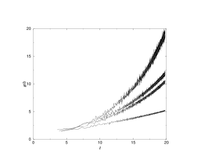
Figure 3.3: Mean length multiplicities of periodic orbits for the Hecke triangles with (from top to bottom) $n=12$, $n=5$, $n=8$, and $n=10$. White lines are numerical fits (3.36).

At Fig. 3.3 we present the numerically computed mean length multiplicities for the Hecke triangles with $n=5,\;8,\;10,\;12$ for lengths $l<20$. White lines indicate a two-parameter fit to these data in the form $\bar{g}(l)=a_{n}e^{b_{n}l}$

$$n = 5\;\;:\;\bar{g}(l)\approx 1.235e^{.114l}\;,$$

$$n = 8\;\;:\;\bar{g}(l)\approx 1.095e^{.114l}\;,$$ (3.36)

$$n = 10\;:\;\bar{g}(l)\approx 1.143e^{.065l}\;,$$

$$n = 12\;:\;\bar{g}(l)\approx.986e^{.150l}\;.$$

These expressions fit numerical data in the given interval of lengths quite well and indicate that for, at least, certain Hecke triangles mean length multiplicity increases exponentially. We stress that (3.36) are only the best least-square numerical fits and no attempts were made to determine the accuracy of coefficients.

The discussion of the origin of such unexpected multiplicities for non-arithmetic triangles is beyond the scope of these lectures (on this subject see unpublished ). However it is of interest to understand why exponentially large multiplicities of periodic orbit lengths do not contradict the observed GOE behaviour of spectral statistics (cf. Fig. 3.2).

Assume that a system has an exponentially large number of periodic orbits with the same length $l$ increasing as

$$g(l)\sim\frac{\mathrm{e}^{\lambda l}}{l}$$

with $\lambda\leq 1/2$.

Let us repeat the arguments of Sect. 1.2 for this case with exact degeneracicies. In Sect. 1.2 it was demonstrated that periodic orbits with different lengths can be treated in the diagonal approximation if

$$l_{p_{1}}-l_{p_{2}}\gg\frac{k}{\Delta E}$$ (3.37)

where $k$ is the momentum and $\Delta E$ is the width of the energy average inherent in the definition of correlation functions of dynamical systems.

As the density of orbits with different lengths is

$$\rho_{\mbox{\scriptsize diff. lengths}}\approx\frac{\mathrm{e}^{l}}{g(l)l}\sim\mathrm{e}^{(1-\lambda)l}$$

it follows that the inequality (3.37) is valid till maximal length

$$l_{m}\sim\frac{1}{1-\lambda}\ln\frac{\Delta E}{k}\sim\frac{1}{1-\lambda}\ln k\;.$$ (3.38)

Notice that due to assumed large multiplicity $l_{m}$ is different from (2.12).

From (3.21) it follows that the two-point correlation form factor in the diagonal approximation up to numerical factor is

$$K(t)\sim\frac{k}{l}|A(l)|^{2}g(l)\mathrm{e}^{l}$$

where $t=l/2k$ and $A(l)\sim l\mathrm{e}^{l/2}/k$. Combining all terms together one obtains that during the maximal time of applicability of the diagonal approximation $t_{m}=l_{m}/2k$ with $l_{m}$ from (3.38) the form factor increases till

$$K(t_{m})\sim\frac{\mathrm{e}^{\lambda l_{m}}}{k}\sim k^{(2\lambda-1)/(1-\lambda)}\;.$$

Hence, if $\lambda=1/2$ as for arithmetic systems the two-point correlation form factor during the time of validity of the diagonal approximation increases till a constant value of the order of 1. But if $\lambda<1/2$ the form factor for the time of validity can reach only a value of the order of $k^{-\nu}$ with $\nu=(1-2\lambda)/(1-\lambda)>0$. As $k\to\infty$ this value tends to zero and no apparent contradiction with standard random matrix ensembles can be derived within the diagonal approximation.

8 Summary

Arithmetic groups are a special sub-class of discrete groups characterized by the existence of a representation by matrices with integer elements. A readable mathematical review of such groups is given in Katok . There are two types of arithmetic groups. The first includes groups commensurable with the modular group and having non-compact fundamental domains with infinite cusps. The second type of compact arithmetic groups combines groups commensurable with groups derived from quaternion algebras with division. These groups have finite fundamental domains.

From classical viewpoint the free motion on surfaces generated by arithmetic groupes is as chaotic as for any hyperbolic surfaces. But quantum mechanics on these arithmetic surfaces is very special. In particular, spectral statistics of the Laplace–Beltrami operator automorphic with respect to arithmetic group is described by the Poisson statistics typical for integrable systems and not by the random matrix statistics typical for chaotic models.

The origin of this peculiarity can be traced to the existence in arithmetic systems of a very large number of periodic orbits with exactly the same length. For all arithmetic groups the mean multiplicity of periodic orbits with length $l$ behaves like $\mathrm{e}^{l/2}/l$. This has to be compared with the total density of periodic orbits which for all discrete groups is $\mathrm{e}^{l}/l$. It is the cumulative effect of the interference of many periodic orbits with the same length which changes drastically the spectral statistics.

In the diagonal approximation the two-point correlation form factor $K(t)$ for arithmetic systems at small $t$ increases exponentially like $\mathrm{e}^{kt}/k$ and during the Ehrenfest time (which is the limit of applicability of the diagonal approximation) reaches a constant value.

More detailed information can be obtained for the modular group where it is possible to compute the two-point correlation form factor analytically. The final answer is

$$K(t)={1\over 2\pi^{2}k}\sum_{(p,q)=1}\left|{q\over p}\beta(p,q)\right|^{2}\delta(t-t_{p,q})$$

where

$$t_{p,q}={1\over k}\ln{kq\over\pi p}$$

and $\beta(p,q)$ is a number-theoretical function given in Sect. 4.3.

This formula means that the two-point form factor for the modular group is a sum over $\delta$-functions at special points $t_{p,q}$ situated in a vicinity of the Ehrenfest time. The set of $\delta$-functions is dense but the largest peaks correspond to the smallest ratios $p/q$. Nevertheless, small peaks with $p/q\ll 1$ are much more numerous and integrally they dominate. In the limit $t$ fixed and $k\to\infty$ $K(t)\to\bar{d}$ thus confirming the Poisson nature of the spectral statistics of the modular group.

Arithmetic groups have many interesting properties. Hecke operators and the Jacquet–Langlands correspondence are the most remarkable.

Acknowledgement

It is a pleasure to thank Charles Schmit for his aid in the preparation of these lectures and A.M. Odlyzko for presenting numerical data of the two-point correlation function of Riemann zeros.

References

• (1) D. Alonso and P. Gaspard, $\hbar$-Expansion for the Periodic Orbit Quantization of Chaotic Systems, Chaos 3 (1993) 601-612; Erratum ibid 4 (1994) 105.
• (2) A.V. Andreev and B.L. Altshuler, Spectral Statistics beyond Random Matrix Theory, Phys. Rev. Lett. 75 (1995) 902-905.
• (3) R. Aurich, M. Sieber, and F. Steiner, Quantum Chaos on the Hadamard-Gutziller problem, Phys. Rev. Lett. 61 (1988) 483.
• (4) A. Aurich and F. Steiner, On the Periodic Orbits of a Strongly Chaotic System, Physica D 32 (1988) 451.
• (5) H.P. Baltes and E.R. Hilf, Spectra of Finite Systems, Wissenschaftverlag, Mannheim, 1976.
• (6) R. Aurich, E. Bogomolny, and F. Steiner, Periodic Orbits on the Regular Octagon, Physica D 48 (1991) 91-101.
• (7) N.L. Balatz and A. Voros, Chaos on the Pseudosphere, Phys. Rep. 143 (1986) 109.
• (8) R. Balian and C. Bloch, Distribution of eigenfrequencies for the wave equation in a finite domain: I Three-dimensional problems with smooth boundary surface, Ann. Phys. 60 (1970) 401; II Electromagnetic Field. Riemannian spaces, Ann. Phys. 64 (1971) 271; III Eigenfrequency density fluctuations, Ann. Phys. 69 (1972) 76; ibid Asymptotic evaluation of the Green’s function for large quantum numbers, Ann. Phys. 63 (1971) 592; ibid Solutions of the Schrödinger equation in terms of classical paths, Ann. Phys. 85 (1974) 514.
• (9) M.V. Berry and M. Tabor, Closed Orbits and the Regular Bound Spectrum, Proc. R. Soc. Lond. A 349 (1976) 101-123.
• (10) M.V. Berry and M. Tabor, Level Clustering in the Regular Spectrum, Proc. R. Soc. London A 356 (1977) 375-394.
• (11) M.V. Berry, Semiclassical Theory of Spectrum Rigidity, Proc. R. Soc. London A 400 (1985) 229-251.
• (12) M.V. Berry, Semiclassical formula for the number variance of the Riemann zeros, Nonlinearity, 1 (1988) 399-407.
• (13) M.V. Berry, Some Quantum-to-Classical Asymptotics, in LesHouches (1989) 251-303.
• (14) M.V. Berry and C.J. Howls, High Orders of the Weyl Expansion for Quantum Billiards, Resurgence of Periodic Orbits, and the Stokes Phenomenon, Proc. R. Soc. Lond A 447 (1994) 527-555.
• (15) M.V. Berry and J.P. Keating, $H=xp$ and the Riemann zeros, in ’Supersymmetry and trace formulas’, eds. I.V. Lerner and J.P. Keating, Plenum, New York (1999) 355-367.
• (16) O. Bohigas, Random Matrix Theories and Chaotic Dynamics, in LesHouches (1989) 87-199.
• (17) O. Bohigas, M.-J. Giannoni, and C. Schmit, Characteristic of Chaotic Quantum Spectra and Universality of Level Fluctuations Law, Phys. Rev. Lett. 52 (1984) 1 ; Spectral Properties of the Laplacian and Random Matrix Theory, J. Physique Lett. 45 (1984) L-1015.
• (18) E. Bogomolny, B. Georgeot, M.J. Giannoni, and C. Schmit, Chaotic Billiards Generated by Arithmetic Groups, Phys. Rev. Lett. 69 (1992) 1477-1480.
• (19) E.Bogomolny and C. Schmit, Semiclassical Computation of High-Excited Energy Levels, Nonlinearity 6 (1993) 523-547.
• (20) E. Bogomolny, Introduction to models on constant negative curvature surfaces, in Quantum Dynamics of Simple Systems, The Forty Fourth Scottish Universities Summer School in Physics, Stirling, 1994, Eds. G-L Oppo, S. M. Barnett, E. Riis, and M. Wilkinson.
• (21) E. Bogomolny and J.P. Keating, Gutzwiller’s Trace Formula and Spectral Statistics: Beyond the Diagonal Approximation, Phys. Rev. Lett. 77 (1996) 1472-1475.
• (22) E. Bogomolny and J.P. Keating, Random Matrix Theory and the Riemann Zeros I: , Nonlinearity 8 (1995) 1115-1131; Random Matrix Theory and the Riemann Zeros II: n-point correlations, Nonlinearity 9 (1996) 911-935.
• (23) E. Bogomolny, F. Leyvraz, and C. Schmit, Distribution of Eigenvalues for the Modular Group, Commun. Math. Phys. 176 (1996) 577-617.
• (24) E. Bogomolny, B. Georgeot, M.-J. Giannoni, and C. Schmit, Arithmetic Chaos, Phys. Rep. 291 (1997) 219-324.
• (25) E. Bogomolny, Spectral Statistics and Periodic Orbits, in Proceedings of the International School of Physics ‘Enrico Fermi’, Varenna (1999), New Directions in Quantum Chaos, Eds. G. Casati, I. Guarneri, and U. Smilansky, IOS Press, Amsterdam, Oxford, Tokyo, Washington, 2000, 333-369.
• (26) E. Bogomolny and C. Schmit, Multiplicities of Periodic Orbits Lengths for Non-Arithmetic Models, (2003) nlin.CD/0312057.
• (27) J. Bolte, G. Steil, and F. Steiner, Arithmetic Chaos and Violations of Universality in Energy Level Statistics, Phys. Rev. Lett. 69 (1992) 2188.
• (28) Chaos and Quantum Physics, Proceedings of the Les Houches Summer School (1989) Eds. M.-J. Giannoni, A. Voros, J. Zinn-Justin. North Holland, Amsterdam, London, New York, Tokyo, 1991.
• (29) Y. Colin de Verdière, Hyperbolic Geometry in Two-Dimensions and Trace Formulas, in LesHouches (1989) 305-330.
• (30) A. Connes, Trace Formula in Non-Commutative Geometry and the Zeros of the Riemann Zeta Function, (1997) arXiv: math.NT/9811068.
• (31) H. Davenport, Multiplicative Number Theory, revised by H. Montgomery, Springer-Verlag, New York, Heidelberg, Berlin, 1980.
• (32) A. Erdélyi et al. Higher Transcendental Functions Vol. 1 (Bateman Manuscript Project). McGraw–Hill, New York, 1953.
• (33) M.C. Gutzwiller, Chaos in Classical and Quantum Mechanics, Springer, New York, 1990.
• (34) J.H. Hannay and A.M. Ozorio de Almeida, J. Phys. A 17 (1984) 3429-3440.
• (35) G.H. Hardy and J.E. Littlewood, Some Problems of ‘Partitis Numerorum’; III: On the expression of a Number as a Sum of Primes, Acta Mathematica, 44 (1923) 1-70.
• (36) G.H. Hardy and E.M. Wright, An Introduction to the Theory of Numbers, Clarenton Press, Oxford, 1979.
• (37) E. Hecke, Lectures on Dirichlet Series, Modular Functions and Quadratic Forms, Vandenhoeck and Ruprecht, Gottingen, 1983.
• (38) D. Hejhal, The Selberg Trace Formula and the Riemann Zeta Function, Duke Math. J. 43 (1976) 441-482.
• (39) D. Hejhal, The Selberg Trace Formula for PSL(2,R), Vol. 1, Lectures Notes in Mathematics 548 (1979); Vol. 2, ibid 1001 (1983).
• (40) D. Hejhal, A classical approach to a well known spectral correspondence on quaternion groups, in Number Theory, D.V. Chudnovsky, G.V. Chudnovsky, H. Cohn, M.B. Nathanson Eds., Lectures Notes in Mathematics 1135 (1985) 127.
• (41) R.D. Horowitz, Characters of Free Groups Represented in the Two-Dimensional Special Linear Group, Comm. Pure Appl. Math. 25 (1972) 635.
• (42) S. Katok, Fuchsian Groups, University of Chicago Press, Chicago and London, 1992.
• (43) J.P. Keating and N.C. Snaith, Random Matrix Theory and $\zeta(1/2+it)$, Commun. Math. Phys. 214 (2000) 57-89.
• (44) A.G. Kurosh, Lectures in General Algebra, Pergamon Press, Oxford, London, Edinburgh, New York, Paris, Frankfurt, 1965.
• (45) H.L. Montgomery, The pair correlation of zeros of zeta-function, Proc. Symp. Pure Math. (1973) 181-193.
• (46) M.L. Mehta, Random Matrices and the Statistical Theory of Energy levels, Academic Press, New York, 1967.
• (47) A.M. Odlyzko, On the Distribution of Spacing Between Zeros of Zeta Function, Math. of Comp. 48 (1987) 273.
• (48) The web site of A.M. Odlyzko: www.dtc.umn.edu/$\sim$odlyzko/.
• (49) A.M. Odlyzko, private communication (2003).
• (50) Manfred Peter, The Correlation Between Multiplicities of Closed Geodesics on the Modular Surface (2001) arXiv: math.NT/0104234.
• (51) B. Randol, The Length Spectrum of Riemann Surface is Always of Unbounded Multiplicity, Proc. Amer. Math. Soc. 78 (1980) 455.
• (52) C. Schmit, Quantum and Classical Properties of Some Billiards on the Hyperbolic Plane, in LesHouches (1989) 331-369.
• (53) K. Takeuchi, On some Discrete Subgroups of SL(2,R), J. Fa. Sci. Univ. Tokyo Sect. 1A 16 (1969) 97-100; A Characterization of Arithmetic Fuchsian Groups, J. Math. Soc. Japan 27 (1975) 600-612; Arithmetic Triangle Groups, J. Math. Soc. Japan 29 (1977) 91-106; Commensurability Classes of Arithmetic Triangles Groups, J. Fac. Sci. Univ. Tokyo Sect. 1A 24 (1977) 201-212.
• (54) A. Terras, Harmonic Analysis on Symmetric Spaces and Applications, Springer, Berlin, 1979.
• (55) E. C. Titchmarsh, The Theory of the Riemann Zeta–Function. Oxford, Clarenton Press, 1951.
• (56) M.F. Vignéras, Arithmetique des algèbres de quaternions, Lectures Note in Mathematics, 800 (1980).