Experimental test of the Gallavotti-Cohen fluctuation theorem in turbulent flows

Abstract

We test the fluctuation theorem from measurements in turbulent flows. We study the time fluctuations of the force acting on an obstacle, and we consider two experimental situations: the case of a von Kármán swirling flow between counter-rotating disks (VK) and the case of a wind tunnel jet. We first study the symmetries implied by the Gallavotti-Cohen fluctuation theorem (FT) on the probability density distributions of the force fluctuations; we then test the Sinai scaling. We observe that in both experiments the symmetries implied by the FT are well verified, whereas the Sinai scaling is established, as expected, only for long times.

I Introduction

The fluctuations of global quantities in out-of-equilibrium systems is a subject of current interest which presents many unsolved problems. One of these problems is the prediction of the shape of the probability density function (PDF) of the variable under study; the PDF is of course not necessarily Gaussian Holdsworth . Among several approaches used to study these problems, the theory of Gallavotti and Cohen galla1 ; galla2 ; galla3 ; Kurchan ; Ramses , based on a chaotic hypothesis, leads to interesting predictions. The main prediction of the Gallavotti- Cohen fluctuation theorem (FT) galla1 concerns the probability density function of a variable related to the phase space contraction rate of the nonequilibrium system under study, this variable being a current $j$ such as the flux of heat, or of momentum, or energy, etc. The mean of $j$ on a time interval $\tau$ is defined as

$$J_{\tau}={1\over\tau}\int_{t}^{t+\tau}j(t^{\prime})dt^{\prime}\ .$$ (1)

One is then interested in the the probability distribution $\pi_{\tau}(Y)$ of the variable $Y=J_{\tau}/J_{\infty}$, where $J_{\infty}=\lim_{\tau\rightarrow\infty}J_{\tau}$ is the stationary average current studied in the system. If $\tau$ is larger than a characteristic time of the system, then the chaotic hypothesis galla1 predicts that $\pi_{\tau}(Y)$ verifies

$$\ln{\pi_{\tau}(Y)\over\pi_{\tau}(-Y)}=\tau\ \sigma\ Y$$ (2)

where $\sigma$ is proportional to the phase space contraction rate. It is important to stress that the above equation is valid for all values of $Y$. A related expression for the probability density $\pi_{\tau}(Y)$ has been established by Sinai under quite general assumptions: $\pi_{\tau}(Y)=A_{\tau}\ e^{-\zeta(Y)\ \tau}$. In this formulation the function $\zeta(Y)$ is a limiting function, for $\tau\rightarrow\infty$,

$$\zeta(Y)={\ln[\pi_{\tau}(Y)]-\ln[A_{\tau}]\over\tau}\ ,$$ (3)

independent of $\tau$ Sinai . However, the FT (with the addition of the chaotic hypothesis) is giving more information: the function $(\zeta(Y)-\zeta(-Y))$ is linear in $Y$ and its derivative is related to the contraction rate in phase space. In this sense, the FT takes into account the underlying dynamics taking place in the system.

However, in the original derivation of the fluctuation theorem, the proof requires several very restrictive hypothesis, among which the time reversibility of the system. Therefore it is important to check the symmetry predicted by eq.2 in more realistic systems in order to probe the universality and applicability in practical cases. Eq.2 has been tested with success on a numerical simulation of a rather artificial system galla4 , and it is also quite well verified for the heat flux in a chain of coupled non-linear oscillators Livi ; Aumaitre and in the energy dissipation rate in the shell model of turbulence Aumaitre .

The situation is less clear for local variables. Gallavotti galla3 suggested that the predictions of the FT could be extended to “the average of local observables”. This has prompted us to check this hypothesis using local measurements in a turbulent flow. We started with preliminary tests using the data of turbulent Rayleigh-Benard convection Cili1 . These tests did show that the fluctuations of a quantity proportional to the heat flux verify both eq.2 and eq.3. In this article we consider the case of the pressure fluctuations in a turbulent wind. Specifically, we consider the statistics of the force applied on an object. We find that its fluctuations verify the Gallavotti-Cohen predictions.

II Experimental apparatus

The experimental set-up which is shown in fig.1 consists of two coaxial, counter rotating disks. This experimental set-up, known as the von Kármán geometry, produces an intense turbulence in a compact region of space. It has been previously used to study the fluctuations of the power injected to maintain the turbulent flow at a fixed integral Reynolds number — more details on the experimental apparatus can be found in ref.PintonI .

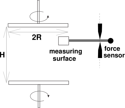
Figure 1: von Kármán experimental set-up. The discs with radius $2R=20$ cm are set $H=20$ cm apart. They are counter rotated at the fixed frequency $\Omega=40$ Hz.

The distance between the disks is 20 cm. As illustrated in fig.1 a square plate, of side 4 cm and 1 mm thick, is inserted between the two disks at a distance of 6 cm from one of the two disks, with its center at 6 cm from the disks rotation axis. The plate is mounted on an extreme of a 10 cm long lever. The other extreme of the lever is fixed on a strain gage (ENTRAN ELFS-T3M-10N force transducer). The lever axis, which is at distance of 1 cm from the strain gage, is mounted on very precise ball bearings in order to reduce friction. With this system the minimum detectable force exerted on the plate is 1 mN, with a response time of $10^{-2}$ s.

The quantity under measurement is the integral of the pressure over the area $S$ of the object:

$$\mathbf{F}(t)=\int_{S}\,ds\;p(\mathbf{r},t)\ .$$ (4)

The pressure itself $p(\mathbf{r},t)$ is the solution of the Poisson equation

$$\Delta p(\mathbf{r},t)=2\rho\partial_{i}u_{j}(\mathbf{r},t)\partial_{j}u_{i}(\mathbf{r},t)\ ,$$ (5)

where $\rho$ is the fluid density and $\partial_{i}u_{j}$ the velocity gradient tensor. It thus instantaneoulsy relates to the strain and vorticity fluctuations in the flow. Note that the presence of the object introduces a no-slip condition on its surface which changes the velocity distribution; the fluctuations of force on the objet are related — but not strictly equal — to the flux of momentum in the undisturbed flow in the absence of the obstacle. The mean value $F_{0}$ of the force on the object is set by the pressure head ($p\simeq\rho U^{2}$), where $U$ is the mean velocity at the location of the object. The time fluctuations of the force are related to the small scale turbulent fluctuations, as indicated by equation (5) and shown in several studies on the fluctuations of the local pressure FauvePression ; CadotPression .

We analyze a set of data recorded at a disk rotation frequency of 40 Hz, corresponding to a Reynolds number of about $Re=2\ 10^{5}$. The signal of the instantaneous force $F(t)$ is filtered at 70 Hz and sampled at 160 Hz with 21bits resolution Agilent 1430 digitizer ($\tau_{0}=1/160=6.25$ ms is the sampling time). The signal is recorded for about $2\ 10^{4}$ integral times. In these conditions the mean force $F_{0}$ on the plate is $0.12$ N.

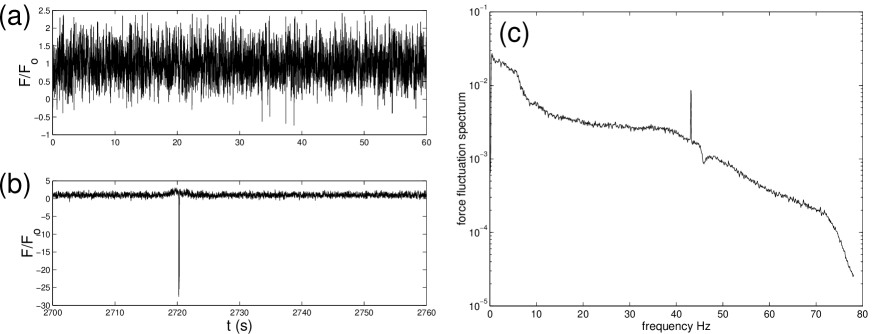
Figure 2: (a) Force of the wind on the measuring surface as a function of time. (b) Expanded view of the force signal — note the strong negative peaks. (c) Power spectrum of the force fluctuations.

The variable of interest is $y=F(t)/F_{0}$. Its typical time evolution is plotted in fig.2; in (a) is shown the ‘standard’ fluctuations of the signal in a large time-window while in (b) we have selected a time interval during which a negative fluctuation of large amplitude occurs. One observes that $y=F(t)/F_{0}$ fluctuates mainly about the mean value $1$, but also that there are strong negative events: sometimes the plate is pushed in the opposite direction of the mean wind velocity. The spectrum, plotted in fig.2(c), is very broad. The thin peak at 40 Hz corresponds to the disk rotation frequency. The cut-off at 70 Hz is imposed by the filter of the digitizer. Note on the spectrum that the change of slope near 35 Hz is at a frequency of the order of $U/L$ where $U$ is the mean velocity at the plate location and $L$ is the plate size.

III Data analysis

The data analysis of the fluctuations of the normalized force $y=F/F_{0}$ has been performed in the following way. We first compute the integrated quantity:

$$Y(t,\tau)={1\over\tau}\int_{t}^{t+\tau}y(t^{\prime})dt^{\prime}\,,$$ (6)

then we calculate the histograms of the $Y(t,\tau)$ values in order to obtain the probability density functions $\pi_{\tau}(Y)$ for each value of the coarse graining time $\tau$. The logarithm of the functions $\pi_{\tau}(Y)$ are plotted in fig.3 as a function of $Y$ for $\tau=3\tau_{0},10\tau_{0}$ and $20\tau_{0}$. One clearly sees that the PDFs change with the integration time $\tau$. For all values of $\tau$, they are non-Gaussian eventhough the force results from a spatial integration of the pressure fluctuations. The central limit theorem does not necessarily apply here BHP because the pressure fluctuations can be correlated over the plate size: they are caused by turbulent structures of sizes ranging from the integral to the dissipative Kolmogorov scale. In addition, one observes the occurence of negative fluctuations, as shown in fig.2.

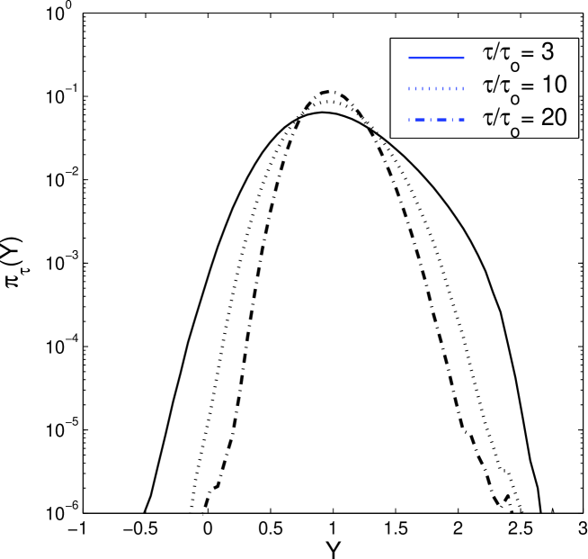
Figure 3: Probability density function for the fluctuations of the force on an obstacle placed in the von Kármán flow, corresponding to the time signals shown in fig.2(a,b)

From the PDF $\pi_{\tau}(Y)$, we construct the function $G_{\tau}(Y)=\ln({\pi_{\tau}(Y)\over\pi_{\tau}(-Y)})$ for $0\leq Y\leq 0.5$. This small interval around zero allows us to study the symmetry of $G_{\tau}(Y)$ even for the largest integration times, e.g. $\tau=20\tau_{0}$. The function $G_{\tau}(Y)$ is plotted as a function of $Y$ in fig.4(a) for $\tau=3\tau_{0},5\tau_{0}$ and $10\tau_{0}$. We find that $G_{\tau}(Y)$ is very much linear in $Y$, as predicted by eq.1 with a slope $\alpha(\tau)$ which increases with $\tau$.

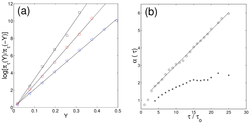
Figure 4: (a) The function $G_{\tau}(Y)$, as defined in the text, plotted as a function of $Y$; integration times: ($\triangle$) $3\tau_{0}$, ($\circ$) $5\tau_{0}$, ($\square$) $10\tau_{0}$. If eq.2 is verified then $G_{\tau}(Y)$ has to be a linear function of $Y$. (b) The function $\alpha(\tau)$ computed using the values $\pi_{\tau}(Y)$ for $-0.5<Y<0.5$ ($\circ$) and $1.5<Y<2.5$ ($\ast$), plotted as a function of $\tau$.

We thus turn to the study of the slope $\alpha(\tau)$ as a function of $\tau$. If eq.1 is correct $\alpha(\tau)$ should be a linear function of $\tau$. The slopes $\alpha(\tau)\;{\rm vs.}\;\tau$ are plotted in fig.4(b). We see that for $\tau/\tau_{0}>4$, the dependence of $\alpha(\tau)$ is linear in $\tau$. It is a quite noteworthy feature that $\tau/\tau_{0}=4$ is very close to the rotation period of the disks (this also corresponds to the correlation time of the von Karman flow BHP ). Indeed, fig.4(b) shows that the linear behaviour of $\alpha(\tau)$, predicted by eq.1, is obtained only for $\tau$ larger than the mean integral time of the system. This observation will be discussed in more details in the next sections.

Here we want to stress another aspect of the measurement, namely the importance of considering the points around $Y=0$ for the study of the Fluctuation Theorem. As a test, we have computed the evolution $\alpha(\tau)$ obtained by the same analysis of the symmetries of the PDF around the point $Y=2$ instead of the point $Y=0$. Corresponding results are plotted with $\ast$ symbols in fig.4(b). We observe that in such a case $\alpha(\tau)$ is not linear in $\tau$. We thus find that the point $Y=0$ has some special property; this is in agreement with the FT prediction.

Summarizing we find that for $\tau/\tau_{0}>4$ $\alpha(\tau)$ is linear, and we can write $\alpha(\tau)=A\tau+B$. Thus

$$\ln{\pi_{\tau}(Y)\over\pi_{\tau}(-Y)}=(A\tau+B)\ Y$$ (7)

We stress that this expression is not in contradiction with eq.1 which has been derived for $\tau\gg\tau_{0}$; rather eq.7 should be considered as a non- asymptotic version of eq.1.

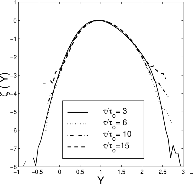
Figure 5: Sinai scaling function obtained from the PDF measured in the counter rotating disk experiment

Finally, we check the existence, for the variable of our experiment, of a function independent of $\tau$ similar to the one defined in eq.3. In order to do this test, we write the PDF as $\pi_{\tau}(Y)=A_{\tau}\ e^{-\zeta(Y)\ \alpha(\tau)}$. Here we use the previously determined function $\alpha(\tau)$ instead of $\tau$, because, as discussed for eq.2, we are not in the asymptotic regime for all values of $\tau$. If the prediction of ref.Sinai can be applied in this case, then $\zeta(Y)=\ln[P(Y)/A_{\tau}]/\alpha(\tau)$ has to be independent of $\tau$. The functions obtained from the PDFs $\pi_{\tau}(Y)$ of fig.3 is plotted in fig.5. We clearly see that the rescaling is very good. In particular we note that the positive part of $\pi_{\tau}(Y)$, which is strongly non-Gaussian, also scales perfectly. Thus the $\alpha(\tau)$ determined using eq.3 allows us to rescale the PDF of $Y$ for any $\tau$. It is important to stress that the rescaling is not possible if $\tau$, instead of $\alpha(\tau)$, is used. Furthermore it is obvious that no scaling can be observed using the $\alpha(\tau)$ obtained by performing the analysis around the point $Y=2$.

In order to check the Sinai scaling function we have performed a different data analysis as suggested in ref. Evans . This analysis, which we will not describe here, yields results in close agreement with those plotted in fig.5.

IV A wind tunnel experiment

In the previous section we have shown that the PDF of the fluctuations of force on a small surface satisfies the symmetries imposed by FT and that they can be rescaled using eq.3. These two properties were also observed on the PDFs of the local heat flux fluctuations in a turbulent thermal convection experiment Cili1 . It is important to recall that eq.2 has been proved for global observables and the fact that the symmetry imposed by eq.2 can be observed on a local measurement is not obvious. In addition, the counter rotating disks experiment and the thermal convection experiment are spatially bounded flows. Indeed, in the von Kármán experiment, one observes that, eventhough the fluid is not confined within walls, the turbulence remains bounded in a volume whose lateral extent is roughly equal to twice the diameter of the driving disks. In such situations, one can argue that a local measurement is indicative of the global behavior of the system.

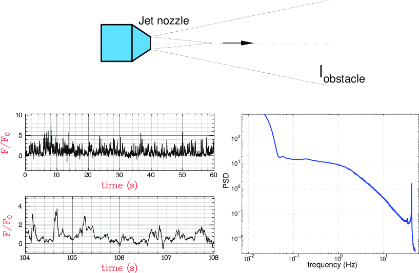
Figure 6: (a) Schematic diagram of the wind tunnel experiment. (b) and (c) Typical time series of the force fluctuations at $Re=45000$. (d) Spectrum of the force fluctuations measured in the wind tunnel at $Re=45000$.

The question thus arises naturally as whether the same observations can be made in truly open systems, where velocity fluctuations are advected outside the observation zone. For this reason, we have repeated the experiment on the wind pressure fluctuations inserting the measuring surface in the turbulent region of a jet developing inside a wind tunnel. The jet is formed by a 5.2 cm nozzle. The obstacle is located 35 diameters downstream of the nozzle where the turbulence is fully developed, at distance of 4 diameters off the axis of the jet. At the measurement location, the mean wind speed is 1 m/s and the Reynolds number based on the jet size is $Re=45000$. The force of the wind on the obstacle is measured as the bending of the shaft that holds the plate, as detected from the deviation of a laser beam. The sampling frequency is $1/\tau_{0}=100$ Hz, and $3.6\ 10^{6}$ data points are accumulated, with a 16 bit resolution.

The force fluctuation spectrum is plotted in fig.6(b). The spectrum is very broad and presents no resonance (the peak at 30Hz is due to the wind tunnel driving fan). As in sec.3 we define the normalized variable $y=F(t)/F_{0}$, and the coarse-grained variable $Y$ after integration over a time interval $\tau$. The PDFs of $Y$ are plotted in fig.7. The curves are extremely non-Gaussian, with the development of an exponential tail at large values of the force, but also important negative excursion on the left-hand side.

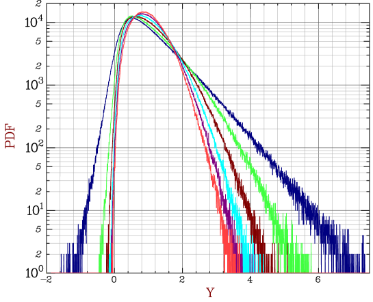
Figure 7: Wind tunnel experiment. PDF of $Y$ for $\tau/\tau_{0}=1,10,20,30,40,50$, upper to lower curve.

In order to analyze them, we repeat on the PDFs of the wind pressure in the wind tunnel the analysis developed in section 3. Specifically we verify that the previously defined function $G_{\tau}(Y)$ is linear in $Y$ for $-0.5<Y<0.5$. In fig.8(a) we plot the measured slope $\alpha(\tau)$ as a function of $\tau$. We find that the affine behavior previously observed, $\alpha(\tau)=A\tau+B$, is again verified here even for small values of $\tau$. It means that the PDFs of the wind tunnel measurements do verify the functional form of the fluctuation theorem (eq.2), in an interval close to $Y=0$.

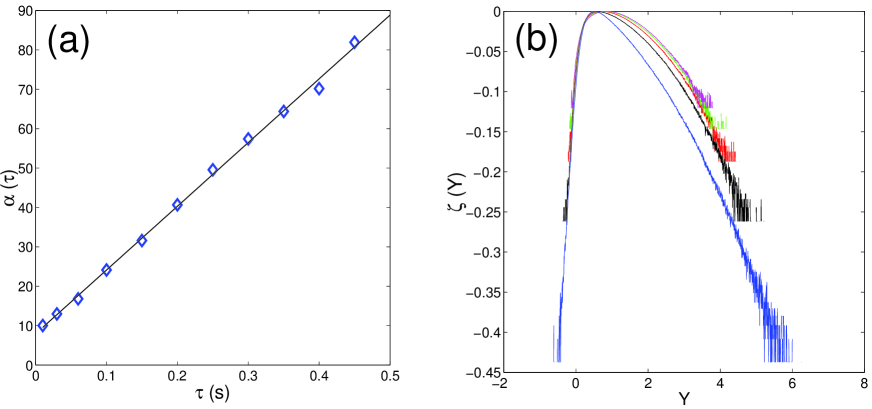
Figure 8: Wind tunnel experiment. (a) $\alpha(\tau)$ and (b) $\zeta(Y)$, estimated as in sec.3

However we find that for small $\tau$ values, it is not possible to derive a unique function $\zeta(Y)$ independent of $\tau$ which would yield a complete rescaling of the PDFs. This is evidenced in fig.8(b) where it can be observed that some rescaling property begins to form at the larges values of $\tau$, e.g. for $\tau>20\tau_{0}$. It is very interesting to note that this time corresponds to the time of flight of the wind from the jet outlet to the measuring point; for times longer than this time of flight, the fluctuations can be associated to global variations of the turbulent field impacting the obstacle, as a block. This point deserves more investigations, some currently under progress.

V Concluding remarks

In this paper we have described two experiments in which we have measured the pressure fluctuations of the wind on a small surface. One of the two experiments, the counter rotating disks, is a spatially correlated flow BHP and the other, the wind tunnel, is an open flow. The main results of this investigation are that in the spatially correlated flow the PDFs of the fluctuations of force on an obstacle, which are strongly non Gaussian, verify the symmetry imposed by the Gallavotti-Cohen fluctuation theorem, and in addition can be rescaled according to the Sinai theory. More precisely in order to rescale the PDF one has to use the measured $\alpha(\tau)$ and not simply $\tau$ as indicated in eq.3. The linear function $\alpha(\tau)$ may be seen as a finite time correction of eq.3, which is valid only for $\tau\rightarrow\infty$. The existence of a scaling function $\zeta(Y)$ independent of $\tau$ is very important because it strengthen the check of the FT. Indeed a strict test of the FT using eq.2 can only be done for values of $Y$ close to zero, and one always observe that the probability of getting negative fluctuations in an actual system is actually very small. However our measurements show that using the value of $\alpha(\tau)$ estimated for $Y$ close to zero, it is possible to scale all the PDFs onto a single function $\zeta(Y)$ for all $Y$. This is a non trivial property which was already observed in the heat fluctuations in turbulent thermal convection Cili1 . This property is not observed, at least for short times, in the jet data described in sec.4 of this paper. The main difference between the jet experiment, the thermal convection and counter rotating disk experiments is that the the first behaves as a spatially uncorrelated flow because perturbations are always advected downstream of the nozzle. As we have already mentioned this difference is an important one. Indeed eq.2 has been proved only for global observables, therefore one can picture that if the turbulence is strong enough, a quasi local measurement can provide a significant measurement of all of the flow, if the later is spatially correlated. This is not necessary true in a open flow where the recurrence time can be very long. This claim is of course preliminary and it merits to be studied in more details.

Another important point which deserves a study is the prefactor in eq.2 which in the standard derivation is the phase space contraction rate. In our experiments we have to study how this prefactor changes as a function of the Reynolds number. This is needed in order to have a more quantitative comparison between theory and experiment.

Finally we have to stress that the study of the probability of extreme negative fluctuations can be very useful in many applications. If one could prove the universality of eq.2 in various geometries, then one would readily use it to compute the probability of the rare, extremely negative, events.

Acknowledgements We acknowledge useful discussions with E. Cohen, G. Gallavotti and L. Rondoni.

References

- (1) Portelli B., Holdsworth P. C.W., Pinton J.-F., Phys. Rev. Lett., 90, 104501 (2003).
- (2) Gallavotti G.,Cohen E.D.G., Phys. Rev. Lett., 74 (1995) 2694-2697.
- (3) Gallavotti G.,Cohen E.D.G., J. Stat. Phys. 80 (1995) 931-970.
- (4) Gallavotti G., Physica D, 112 (1998) 250-257.
- (5) Kurchan J., J. Phys. A , 31, 3719 (1998).
- (6) van Zon R. , E. G. D. Cohen, Phys. Rev. Lett., 91, 110601 (2003).
- (7) Bonetto F., Gallavotti G., Garrido P., Physica D, 105, 226-252, (1997).
- (8) Lepri S., Livi R, Politi A., Physica D, 119, 140 (1998).
- (9) Aumaitre S., Fauve S., McNamara S., Poggi P., Euro. Phys. J. B 19, 449 (2001).
- (10) Gallavotti G., Rondoni L., Segre E., submitted to Physica D, nlin.CD/0209039
- (11) Sinai G. Y., Lectures in Ergodic Theory, Lecture Notes in Mathematics, Princeton University Press, Princeton (1977).
- (12) Ciliberto S., Laroche C., J. Phys. IV France, 8, 6- 215 (1998).
- (13) Labbé R., Pinton J.-F., Fauve S. , J. Phys. II France, 6, 1099 (1996).
- (14) Fauve S., Laroche C., Castaing B., J. Phys. II (France), 3, 271, (1993).
- (15) Cadot O., Douady S., Couder Y., Phys. Fluids, 7(3), 630, (1995).
-
(16)
Bramwell S.T., Holdsworth P.C.W., Pinton J.-F., Nature, 396, 552-
554, (1998).
Pinton J.-F., Labbé R., Holdsworth P.C.W., Phys. Rev. E, 60, R2452-R2455, (1999). - (17) L. Rondoni, G. P. Morris, Open systems and informations dynamics, 10, 105 (2003).