Phaselocked patterns and amplitude death in a ring of delay coupled limit cycle oscillators

Abstract

We study the existence and stability of phaselocked patterns and amplitude death states in a closed chain of delay coupled identical limit cycle oscillators that are near a supercritical Hopf bifurcation. The coupling is limited to nearest neighbors and is linear. We analyze a model set of discrete dynamical equations using the method of plane waves. The resultant dispersion relation, which is valid for any arbitrary number of oscillators, displays important differences from similar relations obtained from continuum models. We discuss the general characteristics of the equilibrium states including their dependencies on various system parameters. We next carry out a detailed linear stability investigation of these states in order to delineate their actual existence regions and to determine their parametric dependence on time delay. Time delay is found to expand the range of possible phaselocked patterns and to contribute favorably toward their stability. The amplitude death state is studied in the parameter space of time delay and coupling strength. It is shown that death island regions can exist for any number of oscillators $N$ in the presence of finite time delay. A particularly interesting result is that the size of an island is independent of $N$ when $N$ is even but is a decreasing function of $N$ when $N$ is odd.

I Introduction

The emergence of self-organized patterns is a common feature of nonequilibrium systems undergoing phase transitions. Examples of such patterns abound in nature ranging from intricate mosaic design on a butterfly wing, vortex swirls in a turbulent stream to synchronous flashing of fireflies [1]. The study of pattern formation and self-synchronization using simple mathematical models consisting of coupled differential equations has therefore been an active area of research spanning many scientific disciplines. For example such models have been employed to examine the collective output of arrays of lasers [2, 3], coupled magnetrons [4], Josephson-junctions [5], coupled chemical reactors [6, 7] and electronic circuits [8]. Rings of oscillators have also been useful for modeling biological oscillations [9, 10] and simulation of phase relations between various animal gaits [11]. These simple discrete models (usually composed of coupled limit cycle oscillators) are amenable to some straightforward analysis and also direct numerical solutions particularly when the number of oscillators is small. When the number of oscillators becomes very large it is often convenient to go over to the continuum limit of infinite oscillators and model the system with a partial differential equation. Examples of the latter are reaction-diffusion type mathematical equations, such as the time dependent complex Ginzburg-Landau equation (CGLE), that have been widely used to simulate the dynamics of pattern formation in fluids and other continuum systems [12]. One of the most popular of the discrete models is the ‘phase only model’ that arose from the pioneering contributions of Winfree [9] and Kuramoto [13, 14]. This model is valid as long as the coupling between the oscillators is assumed to be weak so that amplitude variations can be neglected. When the weak coupling approximation is relaxed and amplitude variations are retained the system is found to admit new collective states such as the amplitude death state [15, 16, 17], chaos and multirhythmicity [18, 19, 20, 21]. This strong coupling model has received a great deal of attention in recent times [17, 22, 23, 24, 11]. The importance of time delay in coupled oscillator systems and its effect on their collective dynamics has been recognized for a long time. In particular there have been a large number of studies devoted to the study of time delay coupled ‘phase only’ models [25, 26, 27, 28, 29, 30, 31, 32, 33, 34]. More recently the strong coupling model has also been generalized to include propagation time delays [35, 36, 37, 38]. A number of interesting results regarding collective oscillations have emerged from this generalized time delayed model some of which have been experimentally verified [39, 40, 41].

Our present work is devoted to further investigations and understanding of the generalized time delay coupled model. Most of the past investigations on this model have been restricted to collective states emerging from global coupling among the oscillators, also known as the mean field approximation. We have chosen to study here the equilibrium and stability of collective modes emerging from a time delay coupled system of identical oscillators in which the coupling is local and restricted to nearest neighbors. The choice of this model is motivated by several considerations. From a basic studies point of view the model offers us an opportunity to compare and contrast the properties of the collective states of the local coupling geometry to that of the globally coupled states. The model further permits a parametric study of the influence of the number of oscillators $N$ on the stability and existence properties of the equilibrium states. In the limit of large $N$ the model also has close resemblance to the continuum CGLE and it is of interest to delineate the important differences in the collective properties of the two systems. From a practical point of view our model has great relevance for many physical systems including coupled magnetrons, study of collective phenomena in excitable media, coupled laser systems, and small-world networks. For example, an interesting study on the role of the geometry of the coupled magnetrons on their rate of phaselocking was made by Benford et al. [4] who experimentally demonstrated production of higher microwave power at Giga Watt levels through phaselocking. Our analysis of nearest neighbor coupled oscillator array could provide important clues on not only the effect of circular geometry but also on the effects of time delay in such a geometry. A ring of coupled oscillators is also commonly encountered in a variety of biological clocks [9]. For simplicity of analysis most mathematical studies of these rings have been confined to an examination of their phase evolutions. Our model analysis can provide an extended understanding of these biological clocks with the inclusion of time delays and amplitude effects. Another interesting and more recent potential application of our work is in the rapidly developing area of small-world networks where the simplest studied configuration is often a ring of oscillators with nearest neighbor connections dominating [42]. A recent study has explored the role of time delays in a ring of connected oscillators with a special focus on small-world networks [34]. We believe that our present study of the ring configuration could help provide further insights in this direction with the incorporation of amplitude effects.

The existence of equilibrium states of locally coupled oscillator systems has been studied in the past using group theoretic methods [43, 44]. We use a plane wave method and investigate both the existence and stability regions of the equilibrium states of the coupled system. We derive a general dispersion relation that can be used to determine the equilibrium states of any number of coupled oscillators. The method is further extended to a linear stability analysis of these equilibrium states. Using this technique we delineate the existence regions of the various equilibrium phase-locked patterns of the coupled system. In the limit of small $N$ and in the absence of time delay our results agree with past findings, but we also find new equilibrium states that have not been noticed before. With time delay the existence regions change in a significant manner and in some of the regimes we observe multirhythmicity. Finally we also examine the nature of the death state in our system in the presence of time delay. Although time delay induced death state in locally coupled identical oscillators has been numerically observed in one of our past studies [35] there has been no systematic analytic investigation of this phenomenon. We carry out such an analysis here and delineate the existence of the death region as a function of the time delay and coupling strength parameters. Our analysis yields an interesting result in that the size of the death island is found to be independent of $N$ (the number of oscillators) when $N$ is even but is a decreasing function of $N$ when $N$ is odd.

The paper is organized as follows. In the next section we present the model equations and briefly discuss their similarities and differences with the continuum model CGL equation. Using the plane wave method we next derive the dispersion relation in Section III and proceed to use it to delineate the possible existence regions of the phase-locked patterns both in the presence and absence of time delay. Section IV is devoted to a linear stability analysis of these states in order to identify their actual existence domain. In Section V we briefly look at the stability of the origin, that is the existence domain of the death state, as a function of the time delay parameter and the coupling strength. Our results are summarized and their implications discussed in the concluding Section VI.

II Model equations

We consider a one dimensional closed chain of delay coupled identical limit cycle oscillators that are close to a supercritical Hopf bifurcation. Assuming the coupling to be linear and of the nearest neighbor kind, we can write down the following set of model equations to describe the time evolution of the oscillator states,

$$\frac{\partial\psi_{j}}{\partial t}=(1+i\omega_{0}-\mid\psi_{j}\mid^{2})\psi_{j}+K[\psi_{j+1}(t-\tau)-\psi_{j}(t)]+K[\psi_{j-1}(t-\tau)-\psi_{j}(t)],$$ (1)

$j=1,\ldots,N$, where $\psi_{j}(=X_{j}+iY_{j})$ is the complex amplitude of the $j^{th}$ oscillator, $K>0$ is the coupling strength, $\tau\geq 0$ is a fixed time delay, and $\omega_{0}$ is the natural frequency of the uncoupled oscillators. The basic nonlinear oscillator we have chosen here is simply the normal form of the supercritical Hopf bifurcation equation truncated to the third order. It is also known as the Stuart-Landau oscillator and has been extensively used in the past as a model equation for studying nonlinear phenomena in fluids, lasers, and Josephson junctions. For example, in the absence of time delay ($\tau=0$), the above set of equations (1) have been used to study the coupled wakes arising from a flow behind an array of equally spaced parallel cylinders [45]. Another interesting connection to past work is the continuum limit for $\tau=0$, where one can introduce a lattice spacing $a$, set $\psi_{j}=\psi(ja)$ in (1), rescale $K$ as $K/a^{2}$ and then let $a\rightarrow 0$ with $ja\rightarrow x$. This reduces Eqs. (1) for $\tau=0$ to the well known complex Ginzburg Landau equation,

$$\frac{\partial\psi(x,t)}{\partial t}=(1+i\omega_{0}-\left|\psi(x,t)\right|^{2})\psi(x,t)+K\frac{\partial\psi^{2}(x,t)}{\partial x^{2}}.$$ (2)

The CGLE has been extensively investigated in the past for its rich equilibrium states and for their applications to a variety of physical situations [46, 47]. In the presence of time delay it is not meaningful to take the continuum limit since $a\rightarrow 0$ would also make the propagation time tend to zero. One can instead take the so called thermodynamic limit by letting $N\rightarrow\infty$ and the chain length $L$ $\rightarrow\infty$, while keeping $a=L/N$ fixed. In such a limit the time delay parameter remains finite and meaningful. The thermodynamic limit also preserves the discrete (in space) character of the evolution equations and therefore the corresponding equilibrium states can differ in character from those obtained from a continuum limit. We will discuss some of these differences in the next section where we derive and analyze the dispersion relation for plane waves for our discrete set of equations (1).

III Dispersion relation for plane waves

We seek plane wave solutions of Eq. (1) of the form,

$$\Psi_{j}=Re^{i(jka+\omega t)},$$ (3)

where $a$ is the distance between any two adjacent oscillators and $k$ is the wave number such that $-\pi\leq ka\leq\pi$. The values of $ka$, which define the phase difference between adjoining oscillators, are further constrained by the periodicity conditions inherent in a closed chain configuration. Since $\psi_{N+1}$ must be identical to $\psi_{1}$ and $\psi_{0}$ must be identical to $\psi_{N}$, we must satisfy the condition $\mathrm{e}^{iNka}=1$. This implies that $Nka=2m\pi$, $m=0,1,\ldots,N-1$, that is,

$$ka=m\frac{2\pi}{N},~{}~{}~{}m=0,1,\ldots,N-1.$$ (4)

These discrete values of $ka$ are one of the defining properties of the various phaselocked states of the coupled set of oscillators. Further characteristics of these states are described by a dispersion relation which can be obtained by substituting (3) in Eq. (1) to give, $i\omega=1+i\omega_{0}-R^{2}+2K\left[\cos(ka)e^{-i\omega\tau}-1\right].$ This leads to

$$\omega = \omega_{0}-2K\sin(\omega\tau)\cos(ka),$$ (5)

$$R^{2} = 1-2K+2K\cos(\omega\tau)\cos(ka).$$ (6)

Equations (5) and (6) which constitute the dispersion relation for plane waves of our model equations can be compared to the corresponding dispersion relation obtained from the CGLE, where we can substitute $\psi(x,t)=R_{CGL}\exp(ikx-i\omega_{CGL}t)$ in (2) to get,

$$\omega_{CGL} = \omega_{0},$$ (7)

$$R_{CGL}^{2} = 1-K(ka)^{2}$$ (8)

where we have replaced $K$ by its scaled value. Equations (7) and (8) can also be recovered from (5) and (6) by setting $\tau=0$ and taking the long wavelength limit of $ka\ll 1$. As we can see there are significant differences in the two dispersion relations. While (5) and (6) are valid for any arbitrary value of $N$, (7) and (8) are strictly valid only in the limit of $N\rightarrow\infty$. The spectrum of $ka$ values are therefore continuous for the latter whereas in the former they assume discrete values that are determined by the magnitude of $N$. For $\tau=0$, Eqs. (5) and (7) become identical, but Eq. (6) reduces to,

$$R^{2}=1-2K+2K\cos(ka)=1-4K\sin^{2}(ka/2).$$ (9)

Using $R^{2}>0$ as the defining condition for the possibility of having a phaselocked state, we see that this region is considerably reduced in the case of the CGLE as compared to the discrete model equations for any given value of the coupling parameter $K$. For example, at $K=1/4$, the discrete model allows all modes from $0$ to $\pi$ to exist, whereas the continuum model has an upper cutoff at $ka=2.0$. For $K>1/4$, cutoff regions also appear for the discrete model and are given by the expression,

$$f_{1}=\cos^{-1}(1-1/2K)<ka<f_{2}=2\pi-\cos^{-1}(1-1/2K)$$

As can be seen from the above expression, for $K>1/4$ the anti-phase locked state ($ka=\pi$) is now no longer a permitted state. With the introduction of time delay, the existence region is not only a function of $ka$ (for a given value of $K$) but also depends on $\omega$ which satisfies the transcendental equation (5). This brings about a significant modification of the existence domains and raises the interesting possibility of enabling many of the previously forbidden modes to exist. Since the dispersion relation now has a transcendental character it also introduces additional branches of collective oscillations. To illustrate some of these modifications we consider a few simple examples. Let $C=\cos(\omega\tau)$. By choosing a value for $C$ and in turn defining $S=\sin(\omega\tau)$, we can immediately get an expression for $\omega$, and the resultant equation for $R^{2}$ defines the stability regions.

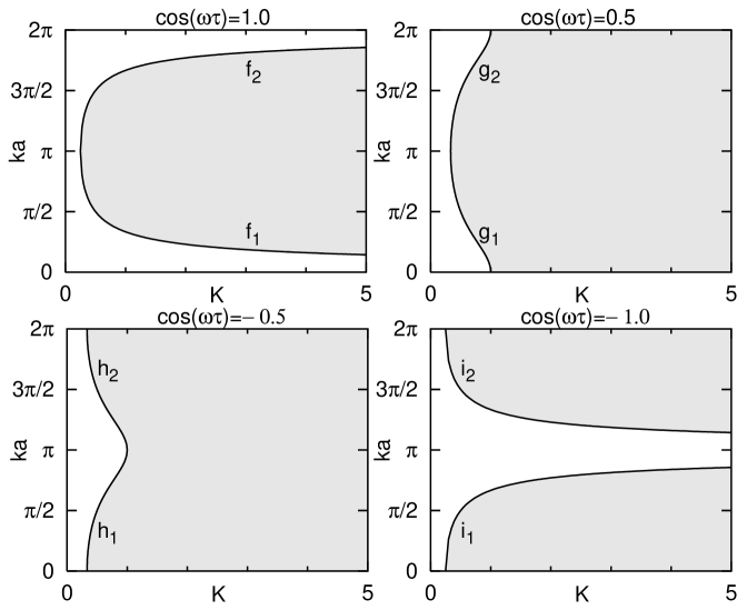
Figure 1: Allowed (unshaded) and forbidden (shaded) wave modes in the presence of time delay for various values of $\cos(\omega\tau)$

Case (i): First let $\cos(\omega\tau)=1.$ This gives $\omega=\omega_{0}$, and the square of the amplitude as $A_{1}=1-2K+2K\cos(ka)$. This also leads us to $\tau=2n\pi/\omega_{0},$ $n=0,1,2,\ldots$. This case also includes the special case of $\tau=0$. Since $A_{1}>0$ for the existence of the solutions, it is easily seen that the bounding region in $(K,ka)$ plane is defined by

$$f_{1}<ka<f_{2}=2\pi-f_{1}$$

where $f_{1}=\cos^{-1}(1-1/2K)$ is the forbidden region. Since $f_{1}$ does not intersect with the $K$ axis at any finite $K$, the region exists for all $K>1/4$. In particular the in-phase state exists for all $K>0$, and the anti-phase locked state ($ka=\pi$) no longer exists if $K>1/4$. This forbidden region is illustrated in Fig. 1(a).

Case (ii): Let $\cos(\omega\tau)=1/2$. This gives the dispersion relation $\omega=\omega_{0}-\sqrt{3}\cos(ka)$. The corresponding delays are defined by $\tau=(2n\pm 1/3)\pi/[\omega_{0}-\sqrt{3}K\cos(ka)],n=0,1,2,\ldots.$ The square of the amplitude is given by $A_{2}=1-2K+K\cos(ka)$. Let $g_{1}=\cos^{-1}(2-1/K)$. The curve $g_{1}$ assumes values for $K$ between 1/3 and 1. If $K>1$, $A_{2}<0$ for any $ka$. So all the modes are forbidden if $K>1$, and the region between $K=1/3$ and $K=1$ as defined by

$$g_{1}<ka<g_{2}=2\pi-g_{1}.$$

is also forbidden. In particular the in-phase solutions do not exist if $K>1$ and the anti-phase solutions do not exist if $K>1/3$. This region is illustrated in Fig. 1(b).

Case (iii): Let $\cos(\omega\tau)=-1/2$. This gives the dispersion relation $\omega=\omega_{0}+\sqrt{3}\cos(ka)$. The corresponding delays are defined by $\tau=(2n\pm 1/3)\pi/[\omega_{0}+\sqrt{3}K\cos(ka)],n=0,1,2,\ldots.$ The square of the amplitude is given by $A_{3}=1-2K-K\cos(ka)$. Let $h_{1}=\cos^{-1}(1/K-2)$. If $K>1$, $A_{3}<0$ for all $ka$. So $K>1$ is the forbidden region. Between $K=1/3$ and $K=1$ the region defined by

$$h_{1}>ka>h_{2}=2\pi-h_{1}$$

is forbidden. The inequality signs are reversed in this case because the curvature of $h_{1}$ is different from that of $g_{1}$ or $f_{1}$. In particular the in-phase solutions are forbidden if $K>1/3$ and the anti-phase solutions are forbidden if $K>1$. This region is illustrated in Fig. 1(c).

Case (iv): Let $\cos(\omega\tau)=-1$. This results in the dispersion relation $\omega=\omega_{0}$ just as in case (i). This case corresponds to $\tau=(2n\pi+1)\pi/\omega_{0},n=0,1,2,\ldots.$ The square of the amplitude is given by $A_{4}=1-2K-2K\cos(ka)$. Since $A_{4}=1$ at $ka=\pi$, in contrast to the three previous cases, the anti-phase locked solutions exist for all values of $K$. At $ka=0$, $A_{4}=1-4K$. So the in-phase solutions are forbidden for all $K>1/4$. The forbidden regions when $K>1/4$ are defined by

$$i_{1}>ka>i_{2}=2\pi-i_{1},$$

where $i_{1}=\cos^{-1}(1/2K-1)$. This region is illustrated in Fig. 1(d). In fact we can derive a general expression for the existence curves by choosing any arbitrary value for $C$. This in turn defines the frequencies as $\omega=\omega_{0}-2KS\cos(ka).$ After some simple algebra, the corresponding delays are given as

$$\tau=(2n\pi+\cos^{-1}C)/[\omega_{0}-2KS\cos(ka)],~{}~{}\mathrm{if}~{}~{}S\geq 0,$$

$$\tau=(2n\pi-\cos^{-1}C)/[\omega_{0}-2KS\cos(ka)],~{}~{}\mathrm{if}~{}~{}S<0.$$

The curve that defines the boundary of the forbidden region is given by $j_{1}=\cos^{-1}(1/S-1/2KS)$ when $S\neq 0$. The case of $S=0$ is the same as case (i) studied above.

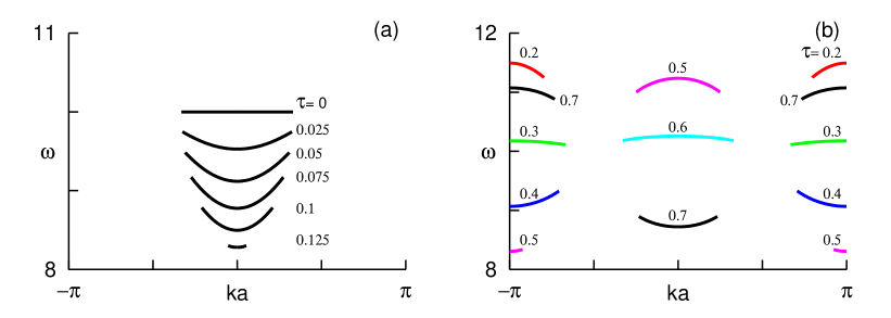
Figure 2: Dispersion relation between allowed wave numbers and the corresponding frequency shown as $\tau$ is gradually increased. $K=1$ and $\omega_{0}=10$. A range of $\tau$ values is forbidden.

Apart from these special cases, the general existence regions are complicated functions of $ka$, $K$ and $\tau$. They need to be determined numerically by simultaneous solution of equations (5) and (6). To demonstrate the constraint imposed by (5) we have plotted its solution ($\omega\;\;vs.\;\;ka$) for various values of $\tau$ and for a fixed value of $\omega_{0}$ and $K$ in Fig. 2(a). When $\tau=0$, the allowed range of $\tau$ is given by abs($ka$)$<\cos^{-1}(1-1/2K)$. So for $K=1$, the phase locked patterns that have wave numbers less than $\pi/3$ are allowed, and all of them have an identical frequency. As $\tau$ is increased the frequency of oscillation decreases for small $\tau$, and the dispersion relation acquires a nonlinear parabolic character. As $\tau$ is further increased, depending on the actual value of $K$, there are bands in $\tau$ values where no modes exist. The shrinking and disappearance of the dispersion curve at $ka=0$ beyond $\tau=0.125$ up to $\tau=0.2$ in Fig. 2(a)-(b) illustrate this phenomenon. One also notices from Fig. 2(b) that at higher values of $\tau$ the dispersion curves become discontinuous and have bands of forbidden $ka$ regions.

IV Stability of phaselocked solutions

We now find the stability of the equilibrium phaselocked solutions discussed in the previous section by carrying out a linear perturbation analysis. Let,

$$\psi_{j}\left(t\right)=\left[R_{k}e^{i\omega_{k}t}+u_{j}\left(t\right)\right]e^{i\left(jka\right)},$$ (10)

where $k=0,1,\cdots,N-1$. Substitution of (10) in Eq.(1), yields in the lowest order the dispersion relation discussed in the previous section. In the next order, where we retain terms that are linear in the perturbation amplitude, we observe that

$$\mid\psi_{k}\mid^{2}\psi_{k}=\cdots+\left[2R_{k}^{2}u_{j}\left(t\right)+R_{k}^{2}e^{2i\omega_{k}t}\bar{u}_{j}\left(t\right)\right]e^{i\left(jka\right)}+\cdots.$$ (11)

Using the above, we obtain the equation

$$\begin{array}[]{rl}\displaystyle{\frac{\partial u_{j}\left(t\right)}{\partial t}}&=\ \ \left(1+i\omega_{0}-2R_{k}^{2}-2K\right)u_{j}\left(t\right)-R_{k}^{2}e^{2i\omega_{k}t}\bar{u}_{j}\left(t\right)\\ &\\ &\ \ \ +K\left[u_{j+1}\left(t-\tau\right)e^{ika}+u_{j-1}\left(t-\tau\right)e^{-ika}\right]\end{array}$$ (12)

and, taking its complex conjugate,

$$\begin{array}[]{rl}\displaystyle{\frac{\partial\bar{u}_{j}\left(t\right)}{\partial t}}&=\ \ \left(1-i\omega_{0}-2R_{k}^{2}-2K\right)\bar{u}_{j}\left(t\right)-R_{k}^{2}e^{-2i\omega_{k}t}u_{j}\left(t\right)\\ &\\ &\ \ \ +K\left[\bar{u}_{j+1}\left(t-\tau\right)e^{-ika}+\bar{u}_{j-1}\left(t-\tau\right)e^{ika}\right].\end{array}$$ (13)

Multiply Eqs. (12) and (13) term-by-term by $e^{i\left(jqa\right)}$, make use of the identities

$$u_{j\pm 1}\left(t-\tau\right)e^{\pm ika}e^{i\left(jqa\right)}=u_{j\pm 1}\left(t-\tau\right)e^{i\left(j\pm 1\right)qa}e^{\pm i\left(k-q\right)a}$$ (14)

and

$$\bar{u}_{j\pm 1}\left(t-\tau\right)e^{\mp ika}e^{i\left(jqa\right)}=\bar{u}_{j\pm 1}\left(t-\tau\right)e^{i\left(j\pm 1\right)qa}e^{\mp i\left(k+q\right)a},$$ (15)

and sum over $j=0,1,2,\cdots,N-1$. Introducing adjoint amplitudes $w_{q}\left(t\right)$ and $\tilde{w}_{q}\left(t\right)$ by the definitions

$$\left[w_{q}\left(t\right),\tilde{w}_{q}\left(t\right)\right]=\sum_{j=0}^{N-1}\left[u_{j}\left(t\right),\bar{u}_{j}\left(t\right)\right]e^{i\left(jqa\right)},$$ (16)

we obtain the set of coupled equations

$$\begin{array}[]{rl}\displaystyle{\frac{dw_{q}\left(t\right)}{dt}}&=\ \ \left(1+i\omega_{0}-2R_{k}^{2}-2K\right)w_{q}\left(t\right)-R_{k}^{2}e^{2i\omega_{k}t}\tilde{w}_{q}\left(t\right)\\ &\\ &\ \ \ +2K\cos\left[\left(k-q\right)a\right]w_{q}\left(t-\tau\right)\end{array}$$ (17)

and

$$\begin{array}[]{rl}\displaystyle{\frac{d\tilde{w}_{q}\left(t\right)}{dt}}&=\ \ \left(1-i\omega_{0}-2R_{k}^{2}-2K\right)\tilde{w}_{q}\left(t\right)-R_{k}^{2}e^{-2i\omega_{k}t}w_{q}\left(t\right)\\ &\\ &\ \ \ +2K\cos\left[\left(k+q\right)a\right]\tilde{w}_{q}\left(t-\tau\right).\end{array}$$ (18)

In order to perform the stability analysis, we assume solutions of the form

$$\left[w_{q}\left(t\right),\tilde{w}_{q}\left(t\right)\right]=\left[ce^{i\omega_{k}t},\tilde{c}e^{-i\omega_{k}t}\right]e^{\lambda t},$$ (19)

which yield the set of coupled equations

$$C_{+}c+R_{k}^{2}\tilde{c} = 0,$$ (20)

$$R_{k}^{2}c+C_{-}\tilde{c} = 0.$$ (21)

In these equations, the quantities $C_{\pm}$ are given by

$$C_{\pm}=\lambda-\left[1\pm i\left(\omega_{0}-\omega_{k}\right)-2R_{k}^{2}-2K\right]-2K\cos\left[\left(k\mp q\right)a\right]e^{\mp i\omega_{k}\tau}e^{-\lambda\tau}.$$ (22)

The eigenvalue equation is obtained from the determinantal condition for Eqs. (20) and (21), namely,

$$C_{+}C_{-}-R_{k}^{4}=0.$$ (23)

This can be expanded to be written in the form of the following characteristic equation,

$$\lambda^{2}+(a_{1}+a_{2})\lambda+(a_{1}a_{2}-R^{4})=0,$$ (24)

where $a_{1}=2R^{2}-1+2K-i(\omega_{0}-\omega)-2K\cos[(k-q)a]{\mathrm{e}}^{-(\lambda+i\omega)\tau}$, $a_{2}=2R^{2}-1+2K+i(\omega_{0}-\omega)-2K\cos[(k+q)a]{\mathrm{e}}^{-(\lambda-i\omega)\tau}$.

It should be noted that the perturbation wave numbers $q$ are once again a discrete set and from the periodicity requirement they obey the relation,

$$qa=m\frac{2\pi}{N},~{}~{}~{}m=0,1,\ldots,N-1.$$

Thus in our stability analysis any pattern corresponding to a given value of $ka$, we need to examine the eigenvalues of Eq. (24) at each of the above permitted values of $qa$. We now proceed to discuss the stability of the various phaselocked patterns both in the absence and presence of time delay.

IV.1 Stability of phaselocked patterns in the absence of delay

In the absence of time delay, the eigenvalue equation (24) can be solved analytically to give,

$$\lambda=1-2R^{2}-2K+2K\cos(ka)\cos(qa)\pm\sqrt{4K^{2}\sin^{2}(ka)\sin^{2}(qa)+R^{4}}.$$ (25)

The real parts of the eigenvalues of Eq. (24) will be negative if $a_{1}+a_{2}>0$ and $a_{1}a_{2}-R^{4}>0$ simultaneously. The first of these conditions can be simplified to give

$$a_{1}+a_{2}=2\left[1-2K\left\{1-\cos(ka)[2-\cos(qa)]\right\}\right]>0,$$ (26)

and the second condition can be simplified to give

$$a_{1}a_{2}-R^{4}=[1-\cos(qa)]4K\left[K\left\{4\cos^{2}(ka)-2\cos(ka)-[1+\cos(qa)]\right\}+\cos(ka)\right]>0.$$ (27)

In the following, we use these two conditions, or, in the simplest cases, the eigenvalue equation itself to determine the stability.

IV.1.1 In-phase patterns ($k=0$ mode)

From the previous section the $k=0$ solution is given by $\omega=\omega_{0}$ and $R=1$. Substituting these in Eq. (25) above, and setting $k=0$, we get,

$$\lambda=\cases{-2K[1-\cos(qa)]\leq 0,\cr-2-2K[1-\cos(qa)]<0,}$$

Thus the plane wave solution $\Psi_{j}(t)=\mathrm{e}^{i\omega_{0}t}$, which is nothing but an in-phase locked solution of the coupled identical oscillators, is stable for $\tau=0$ for all values of $\omega_{0}$.

IV.1.2 Anti-phase patterns ($ka=\pi$ mode)

The equilibrium pattern in this case consists of adjacent oscillators remaining $\pi$ out-of-phase at all times and oscillating with the same frequency $\omega_{0}$. The amplitude of the oscillations is given by,

$$R^{2}=1-4K.$$

As discussed in the previous section, the condition $R^{2}>0$ permits the existence of this mode in the region of $K<1/4$. However as we will see below, using conditions (26) and (27), these permitted anti-phase states are linearly unstable for any arbitrary number of oscillators. Inserting $ka=\pi$ in (26) and (27) the conditions simplify to,

$$K<\mathrm{min}\frac{1}{2[3-\cos(qa)]},$$ (28)

and

$$K>\mathrm{max}\frac{1}{5-\cos(qa)}.$$ (29)

where the $qa$ values are to be determined as per the prescription discussed in the previous section. As simple examples, for $N=2$ the only permitted values of $qa$ are $0$ and $\pi$ and from (28) and (29) above, we arrive at the requirement that $K<1/8$ and $K>1/4$ which is not possible. Hence the mode is unstable. Such conditions were previously obtained by Aronson et al. [16] in their investigation of the collective states of two coupled limit cycle oscillators. In fact, the argument can be extended to any arbitrary even $N$ since

$$5-\cos(qa)\leq 2[3-\cos(qa)]$$

for all values of $qa$ and hence the conditions (28) and (29) cannot be satisfied simultaneously for any value of $K$. This implies that the anti-phase states, characterized by $ka=\pi$, are unstable for any arbitrary value of even $N$.

Figure 3: The contours of $a_{1}+a_{2}=0$ (thin lines), and that of $a_{1}a_{2}-R^{4}=0$ (thick lines). The thin $+$ and $-$ signs indicate the sign of $a_{1}+a_{2}$ in the connected regions bounded by the thin curves, and the thick signs indicate the sign of $a_{1}a_{2}-R^{4}$ in those bounded by the thick curves.

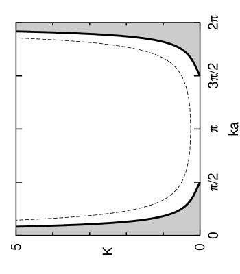
Figure 4: The stability region of the phaselocked states (shaded region which is below $K=K^{\star}$) plotted in $(K,ka)$ space. The left half of the dashed curve is $f_{1}$ and the right half is $f_{2}$ as drawn in Fig. 1(a).

Figure 5: Multiple stable phaselocked patterns for $N=50$ at $\omega_{0}=10$ and $K=0.4$ in the absence of time delay. The real parts of the complex vector $Z_{j}(t)$ are plotted in gray scale.

IV.1.3 Other phaselocked patterns ($k>0$)

Another interesting phaselocked pattern is the $k=\pi/2$ mode. It can be shown by using the conditions discussed above that this pattern is also always unstable. However, a large number of other modes whose wave numbers are close to either $0$ or $2\pi$ are likely to be stable. They coexist with the in-phase stable solutions ($ka=0$). The relations (26) and (27) provide sufficient conditions to find the stability of any given mode. The contours of $a_{1}+a_{2}=0$, and $a_{1}a_{2}-R^{4}=0$, are given, respectively, by

$$qa=\left\{\cos^{-1}[2-(2K-1)/2KC],2\pi-\cos^{-1}[2-(2K-1)/2KC]\right\},$$

$$qa=\left\{\cos^{-1}\left[C(1/K-2+4C)-1\right],2\pi-\cos^{-1}\left[C(1/K-2+4C)-1\right]\right\},$$

where $C=\cos(ka)$. These curves are plotted in Fig. 3 for $K=0.4$. We see that there is a large range of $ka$ values that satisfies the conditions (26) and (27). For a given number $N$ of oscillators if the $ka$ values fall in this range then the corresponding phaselocked patterns are stable. The x-axis intersections of the curve $a_{1}a_{2}-R^{4}=0$ that are closer to $0$ and $2\pi$ provide boundaries of $K$ below which the modes are stable. By setting $qa=0$ in (27), we obtain the condition on $K$ for stability as a function of $ka$:

$$K<\frac{-\cos(ka)}{2[2\cos^{2}(ka)-\cos(ka)-1]}\equiv K^{\star}.$$ (30)

This stability region is plotted in Fig. 4. In the limit of $N\rightarrow\infty$, a continuous range of $ka$ modes are accessible, and the system truly possesses infinitely many stable phaselocked states when $K<K^{\star}$. The stability of these phaselocked solutions is one important result of our paper. Note that all phaselocked patterns with wave numbers between $\pi/2$ and $3\pi/2$ are unstable. We also note from Fig. 4 that for a given value of $K$ it is possible to have more than one stable state corresponding to different values of $ka$ that lie in the two stable regions. In the limit of $N\rightarrow\infty$ such a multistability phenomenon can occur over a continuous range of $ka$ values spanning the stable regions. A numerical example of the multistability of some of these modes is illustrated in Fig. 5 for $N=50$ oscillators at a fixed value of $K=0.4$. By giving initial conditions close to the modes $ka=2\pi/50$, $4\pi/50$, and $6\pi/50$, the corresponding phaselocked solutions are realized.

Now we address the following question: What is the minimum number of oscillators for which a second phaselocked pattern (the first one being in-phase) can become stable? Since the permissible $ka$ values are related to the number of oscillators $N$ in an inverse fashion due to the periodicity requirement (see Eq. (4)) we need to determine the maximum stable $ka$ in order to find the minimum critical $N$. Since $K=K^{\star}$ makes an intersection at $ka=\pi/2$ and $ka=3\pi/2$, the second stable phaselocked pattern that could emerge at this point will have

$$ka=m\frac{2\pi}{N}=\frac{\pi}{2}.$$

Hence $N\geq 4$ for a second phaselocked pattern to ever become stable. Thus for $N=2$ or $N=3$ coupled identical oscillators we will only have in-phase oscillations as stable oscillations and there will not be any other stable phaselocked states. The minimum number of oscillators necessary for multistable behavior is four. Thus $N=4$ is a critical number.

IV.2 Phaselocked patterns for finite time delay

Now we study the synchronized patterns that could become stabilized by the presence of time delay. We noted before that, in the absence of time delay, the in-phase oscillations are always stable, and the anti-phase oscillations are always unstable for any positive finite $K$. Time delay changes the scenario and could make each of these branches stable in certain ranges of $\tau$. In addition, the number of multiple branches of each of these two oscillations increases with $\tau$. Equations (5-6) define the amplitudes and frequencies of these synchronized states. and the characteristic equation (24) determines their linear stability.

Figure 6: The in-phase ($ka=0$) locked frequencies and amplitudes represented by Eq. (1) at $K=10$, and $\omega_{0}=10$. The dashed portions represent the unstable branches for the case of $N=2$ and the continuous lines represent the stable branches.

Figure 7: The anti-phase ($ka=\pi$) locked frequencies and amplitudes represented by Eq. (1) at $K=10$, and $\omega_{0}=10$. The dashed portions represent the unstable branches for the case of $N=2$ and the continuous lines represent the stable branches.

We begin with a simple example of two coupled oscillators, $N=2$, which can have just two phaselocked states, namely in-phase states with $ka=0$ and anti-phase states with $ka=\pi$. We evaluate the eigenvalues for these two cases for different values of $\tau$ by numerically solving Eq. (24) for the permitted values of $qa$ and also confirm the existence of the modes by an actual integration of the original equations. We show the stable (continuous) and unstable (dashed lines) branches of these two solutions in Figs. 6 and 7. A stable in-phase branch emerges from $\tau=0$ and its amplitude becomes $0$ while its frequency is finite showing a supercritical Hopf bifurcation. The first branch of the anti-phase locked state emerges from zero again in a supercritical Hopf. As $\tau$ is increased multiple Hopf bifurcation points are seen. Such stability of the in-phase and anti-phase oscillations were earlier studied by us experimentally using coupled electronic oscillators [40].

Figure 8: Real part of the eigenvalues as a function of $qa$ for $N=10$ at $\omega_{0}=10$, $K=10$, $ka=\pi$, and $\tau=0.2$.

As a second illustration, we consider the case of $N=10$, $\tau=\pi/\omega_{0}$ (i.e. $\cos(\omega\tau)=-1.0$), whose equilibrium existence domain we have discussed earlier as case (iv) in Section III. In particular we have noted that the $ka=\pi$ state is a permitted equilibrium state. To examine its stability we observe that we need to examine the eigenvalues for $qa=m\frac{2\pi}{N},~{}~{}~{}m=0,1,\ldots,N-1$. In Fig. 8 we have plotted the real part of the eigenvalues for all these perturbation wave numbers. We see that they are all negative, which indicates stability of the pattern. In fact, in this case, due to the symmetry of the characteristic equation we can predict stability for all higher values of $N$ as well with the eigenvalues of all additional $qa$ values falling on the dotted line shown in the figure. The existence regions for this case were shown in Fig. 1(d). By considering this case for all the possible values of $qa$ between $0$ and $2\pi$, we are essentially determining the stability of this case in the infinite oscillator limit. We show our numerical results for this case in Fig. 9. It is obtained by tracking the eigenvalue transitions for $qa$ between $0$ and $2\pi$. This phase diagram is strictly true for $N\to\infty$. As can be seen, finite $\tau$ increases the number of stable modes for any given value of $K$. We finally show in Fig. 10 a numerical example of the anti-phase oscillations using $N=50$ oscillators.

Figure 9: (a) Critical boundaries below which stable phaselocked patterns exist are shown for the case of $\cos(\omega\tau)=1$ as $N\to\infty$. (b) Stability region of phaselocked patterns for $\cos(\omega\tau)=-1$ as $N\to\infty$.

Figure 10: Anti-phase locked state of identical oscillators for $N=50$ at $K=10$ and $\tau=0.3$.

V Amplitude death for finite time delay

As is well known, a system of identical oscillators that are globally coupled do not have an amplitude death state [16] but the presence of time delay in the coupling can bring about such a collective state. This phenomenon was first pointed out for two coupled oscillators in [35] and also generalized to $N$ globally coupled oscillators [36]. A similar statement also holds for locally coupled oscillators as will be shown. The death state in the presence of time delay had earlier been numerically confirmed for a finite number of locally coupled oscillators [35]. However no systematic study of the dependence of the death island regions on the magnitude of the time delay and the number of oscillators has so far been carried out for systems of locally coupled oscillators. In this section we address this issue and study the stability of the origin for our discrete model equation (1). Amplitude death state is characterized by $R=0$. To derive an appropriate set of eigenvalue equations for determining the stability of this state, we carry out a linear perturbation analysis about the origin. Substituting ($\psi_{j}=0+\tilde{\psi}_{j}$) in Eq. (1), and discarding the nonlinearities, we get,

$$\frac{\partial\tilde{\psi}_{j}}{\partial t}=(1+i\omega_{0})\tilde{\psi}_{j}+K[\tilde{\psi}_{j+1}(t-\tau)-\tilde{\psi}_{j}(t)]+K[\tilde{\psi}_{j-1}(t-\tau)-\tilde{\psi}_{j}(t)],$$ (31)

where $j=1,\ldots,N$ with periodic boundary conditions. By letting $\tilde{\psi}(t)\propto\mathrm{e}^{i\lambda t}$, the eigenvalue matrix in circulant form is obtained. The determinant of this matrix is written as

$$\prod_{j=1}^{N}\left(\lambda+2K-1-i\omega_{0}-Ke^{-\lambda\tau}U_{j}-Ke^{-\lambda\tau}U_{j}^{N-1}\right)=0,$$

where $U_{j}=\mathrm{e}^{i2\pi(j-1)/N}$ are the $N^{th}$ roots of unity. But $U_{j}+U_{j}^{N-1}=U_{j}+U_{j}^{-1}=2\cos[(j-1)2\pi/N]$. So the above equation takes the form of

$$\prod_{j=1}^{N}\left(\lambda+2K-1-i\omega_{0}-2K\cos[(j-1)2\pi/N]\mathrm{e}^{-\lambda\tau}\right)=0.$$ (32)

The complete set of eigenvalue equations includes the second set obtained by considering the conjugate equation of the above. Note that for $\tau=0$ the above eigenvalue equation (32) always admits at least one unstable eigenvalue, namely $\lambda=1+i\omega_{0}$. Hence identical oscillators that are locally coupled cannot have an amplitude death state in the absence of time delay. We will now determine the amplitude death regions for finite values of $\tau$. We define a factor $R_{j}=2\cos[(j-1)2\pi/N]$ that we will use in the critical curves derived below. If the number of oscillators is a multiple of $4$, there are some eigenvalue equations that emerge without a dependence on $\tau$, when $R_{j}=0$. For example, consider the case of $N=4$ and $j=2,4$. Then, the eigenvalue equation becomes: $\lambda=1-2K\pm i\omega_{0}$. For this equation, the only criticality is given by $K=1/2$. The stable region lies on the side of the parameter space that obeys $K>1/2$. For other values of $R_{j}$, the death island boundaries can be derived by setting the real part of the eigenvalue to zero, and appropriately choosing the signs of the multiple curves that result. The analysis is similar to the one we presented in the treatment of globally coupled oscillators [35, 36], and here we simply provide the final expressions for the critical curves in $(\tau,K)$ plane:

$$\tau_{a}(n,K)=\cases{\frac{2n\pi-\cos^{-1}[(2K-1)/KR_{j}]}{\omega_{0}+\sqrt{K^{2}R_{j}^{2}-(2K-1)^{2}}},~{}~{}~{}R_{j}>0,\cr\frac{(2n+1)\pi-\cos^{-1}[(2K-1)/K\left|R_{j}\right|]}{\omega_{0}+\sqrt{K^{2}R_{j}^{2}-(2K-1)^{2}}},~{}~{}~{}R_{j}<0,}$$ (33)

$$\tau_{b}(m,K)=\cases{\frac{2m\pi+\cos^{-1}[(2K-1)/KR_{j}]}{\omega_{0}-\sqrt{K^{2}R_{j}^{2}-(2K-1)^{2}}},~{}~{}~{}R_{j}>0,\cr\frac{(2m+1)\pi+\cos^{-1}[(2K-1)/K\left|R_{j}\right|]}{\omega_{0}-\sqrt{K^{2}R_{j}^{2}-(2K-1)^{2}}},~{}~{}~{}R_{j}<0.}$$ (34)

$n$ and $m$ are whole numbers. We now determine some useful bounds on $K$ for ordering and finding the degeneracies of the critical curves. The argument of inverse cosine functions and the square root term in the denominators of the above expressions impose the following bounds on $K$:

$$K>1/4,~{}~{}\mathrm{for}~{}~{}R_{j=1},$$ (35)

$$\frac{1}{2+R_{j}}<K<\frac{1}{2-R_{j}},~{}~{}\mathrm{for}~{}~{}R_{j>1}.$$ (36)

The sign of the derivative with respect to $\tau$ of the real part of the eigenvalue is determined by the term $-\mathrm{Im}(\lambda)KR_{j}\sin[\mathrm{Im}(\lambda)\tau]$, and after some algebra it is expressed as

$$\frac{d\mathrm{Re}(\lambda)}{d\tau}\Bigg{|}_{\mathrm{Re}(\lambda)=0}\cases{>0,~{}~{}\mathrm{on}~{}~{}\tau_{a},~{}~{}\mathrm{for~{}any}~{}\omega_{0},\cr<0,~{}~{}\mathrm{on}~{}~{}\tau_{b},~{}~{}\mathrm{if}~{}~{}\omega_{0}>\sqrt{K^{2}R_{j}^{2}-(2K-1)^{2}},\cr>0,~{}~{}\mathrm{on}~{}~{}\tau_{b},~{}~{}\mathrm{if}~{}~{}\omega_{0}<\sqrt{K^{2}R_{j}^{2}-(2K-1)^{2}}.}$$ (37)

The first condition involving $\omega_{0}$ in the above relation leads to the following bounds on $K$:

$$K<(1+\omega_{0}^{2})/4,~{}~{}\mathrm{for}~{}~{}R_{j=1},$$ (38)

$$K>\frac{2+R_{j}\sqrt{1+\omega_{0}^{2}}}{4-R_{j}^{2}},~{}~{}\mathrm{or,}~{}~{}K<\frac{2-R_{j}\sqrt{1+\omega_{0}^{2}}}{4-R_{j}^{2}},~{}~{}\mathrm{for}~{}~{}R_{j>1}.$$ (39)

The ranges of $K$ imposed by the relations (35) and (39) are mutually exclusive. Hence, on the curve $\tau_{b}$ the only boundary across which an eigenvalue pair makes a transition to the negative eigenvalue plane occurs when $R_{j=1}$, and across the curves occurring when $R_{j>1}$, the eigenvalue pair makes a transition to the positive plane. So $\tau_{b}(0,K)$ at $R_{j=1}$ always remains as the left hand side boundary of the death island. In order to see the degeneracy among the curves, note that

$$R_{k}=R_{j},~{}~{}\mathrm{if~{}~{}}k=N+2-j.$$

Also the sign of $R_{j}$ does not play a role in distinguishing the critical curves. These two properties are responsible for a reduction of the number of the actual distinct boundaries of the death islands. These degeneracies can be framed into two cases. First, when $N$ is odd. The total number of distinct values of $R_{j}$ is $(N+1)/2.$ $R_{1}(=2)$ is the maximum of all the $R_{j}$, and is non-degenerate. And $R_{i}$, where $i=2,\ldots,(N+1)/2$ are the other distinct values, whose values are identically equal to $R_{k}$, where $k=N+2-i$. Among the latter $R_{j}$ values, the maximum negative value occurs at $j=(N+1)/2$. The curves corresponding to $R_{j}>0$ and $R_{j}<0$ form the boundaries for two different death islands, as can be seen from the indexes in Eqs. (33-34). A further ordering of the curves must be done by a numerical plotting of the curves. The ordering reveals that for $N\leq 13$, the first death island is bounded by the curves

$$\gamma_{1} : ~{}\tau_{b}(0,K)~{}~{}\mathrm{at}~{}~{}R_{j=1},$$

$$\gamma_{2} : ~{}\tau_{b}(0,K)~{}~{}\mathrm{at}~{}~{}R_{j=(N+1)/2},~{}~{}\mathrm{and}~{}~{}$$

$$\delta_{1} : ~{}\tau_{a}(0,K)~{}~{}\mathrm{at}~{}~{}R_{j=(N+1)/2},$$

$$\delta_{2} : ~{}\tau_{a}(1,K)~{}~{}\mathrm{at}~{}~{}R_{j=1}.$$

The curves $\gamma_{1}$ and $\delta_{2}$ form, respectively, the left and the right boundaries of the death island region. And $\delta_{1}$ and $\delta_{2}$ form the bottom two curves. The existence range along $K$ of $\delta_{1}$, across which the eigenvalues make a transition to the left half plane, increases with increasing $N$. In fact it intersects with $\gamma_{1}$. So this provides the first boundary across which stability is lost. This occurs for $N\geq 15$, when the death island is bounded by the two curves:

$$\gamma_{1} : ~{}\tau_{b}(0,K)~{}~{}\mathrm{at}~{}~{}R_{j=1},~{}~{}\mathrm{and}$$

$$\delta_{1} : \tau_{a}(0,K)~{}~{}\mathrm{at}~{}~{}R_{j=(N+1)/2}.$$

Figure 11: Death islands at $\omega_{0}=10$. All even number of oscillators have a single death island region that is independent of the number of oscillators. The odd number of oscillators are bounded by four curves when $N\leq 13$, and two curves otherwise. These two curves merge in the infinite limit with the curves that represent the even number of oscillators.

Second, when $N$ is even, many more curves become degenerate. The number of distinct value of $R_{j}$ is $N/2+1.$ Among these distinct values, the magnitudes of pairs of them can become identical. If $N$ is divisible by $4$, such pairs are $N/4+1$ in number, and $(N+2)/4$ otherwise. Every positive $R_{j}$ has its negative counterpart. The maximum value of $R_{j}=2$ that occurs when $j=1$, and the next maximum value is at $R_{j=2}$. Hence the equations (33-34) can be simplified to

$$\tau_{c}(n,K)=\frac{n\pi-\cos^{-1}[(2K-1)/KR_{j}]}{\omega_{0}+\sqrt{K^{2}R_{j}^{2}-(2K-1)^{2}}},~{}~{}~{}R_{j=1,\ldots,J},$$ (40)

$$\tau_{d}(m,K)=\frac{m\pi+\cos^{-1}[(2K-1)/KR_{j}]}{\omega_{0}-\sqrt{K^{2}R_{j}^{2}-(2K-1)^{2}}},~{}~{}~{}R_{j=1,\ldots,J},$$ (41)

where $J=N/4+1$ if $N$ is divisible by $4$, and $(N+2)/4$ otherwise. The actual ordering, however, reveals that the death island boundaries are given by $\tau_{c}(0,K)$ at $R_{j=1}$ and $\tau_{d}(1,K)$ at $R_{j=1}$, which are identical, respectively, to $\delta_{1}$ and $\gamma_{1}$. These curves are plotted in Fig. 11. As is seen for $N$ even there is a single death region. In the case of $N$ odd the boundary of the death region depends on the value of $N$. As $N$ increases, the area of the death region decreases. As $N\rightarrow\infty$ the area of the death island for $N$ odd decreases and approaches, as a limit, the boundary for $N$ even. For all $N$, the intersections of $\gamma_{1}$ and $\delta_{1}$ or those of $\gamma_{2}$ and $\delta_{2}$ occur for $K>1/2$. So the delay-independent eigenvalue equations that are mentioned earlier do not contribute to the death island boundaries. The differences in the death island boundaries for even and odd numbered oscillators can be traced primarily to the behavior of the eigenvalues of the lowest permitted perturbation wave numbers. For an even number $N$ of oscillators the smallest perturbation mode is $qa=\pi$. The values of the real parts of the eigenvalues corresponding to this mode are close in their magnitude to those corresponding to the $qa=0$ perturbation mode. Across the right hand side boundary of the death island region, the $qa=\pi$ mode grows positive and the system emerges out of the death region with an anti-phase state. When $N$ is odd, however, the smallest perturbation mode is $qa=\pi-\pi/N$ which is more heavily damped than the $qa=0$ mode. So the death region continues to exist for larger $\tau$ values. Ultimately, the second eigenvalue branch of the $qa=0$ mode (which exists due to the transcendental nature of the eigenvalue equation) grows and the system emerges across the boundary with an in-phase state of a different frequency. As $N$ becomes large, the smallest perturbation mode for the $N$ odd case gets closer to $\pi$ and the death island boundaries of the two cases, as seen in Fig. 11, become indistinguishable. We have independently verified the death regions depicted in Fig. 11, including their interesting dependence on $N$, by a direct numerical solution of (1) over the specified range of parameters. We also illustrate in Fig. 12 an example of the amplitude death state for a chain of $N=50$ oscillators.

Figure 12: Amplitude death of identical oscillators for $N=50$ at $K=10$ and $\tau=0.1$.

VI Discussion and conclusions

We have studied the existence and stability of phaselocked patterns and amplitude death states in a closed chain of delay coupled identical limit cycle oscillators that are near a supercritical Hopf bifurcation. The coupling is limited to nearest neighbors and is linear. The coupled oscillators are modeled by a set of discrete dynamical equations. Using the method of plane waves we have analyzed these equations and obtained a general dispersion relation to delineate the existence regions of equilibrium phaselocked patterns. We have also studied the stability of these states by carrying out a linear perturbation analysis around their equilibria. Our principal results are in the form of analytic expressions that are valid for an arbitrary number of oscillators $N$ (including the $N\rightarrow\infty$ thermodynamic limit) and that can be used in a convenient fashion to identify and or obtain stable equilibrium states for a given set of parametric values of time delay, coupling constant, wave number and wave frequency. We have carried out such an exercise for a number of illustrative cases both with and without the presence of time delay. In the absence of time delay, our analysis reveals a number of new phase-locked states close to the in-phase stable state which can exist simultaneously with the in-phase state. The minimum number of oscillators for which this multirhythmic phenomena can occur is $N=4$. Time delay introduces interesting new features in the equilibrium and stability scenario. In general we have found that time delay expands the range of possible phaselocked patterns and also extends the stability region relative to the case of no time delay. The dispersion curves for varying values of time delay also display some novel features such as forbidden regions and jumps in the range of allowed wave numbers as well as forbidden bands in the space of time delay.

We have also carried out a detailed analytic and numerical investigation of the existence of stable amplitude death states in the closed chain of delay coupled identical limit cycle oscillators. The results not only confirm our earlier numerical demonstration of the existence of such death states but go beyond to provide a comprehensive picture of the existence regions in the parameter space of time delay and coupling strength. The analytic results also establish that death island regions exist for any number of oscillators $N$ for appropriate vales of $K$, $\omega$ and $\tau$. In this sense our work provides a generalization of the earlier amplitude death related results, that were obtained for globally coupled oscillators to the case of locally coupled oscillators. An interesting new result, arising from the local coupling configuration, is that the size of a death island is independent of $N$ when $N$ is even but is a decreasing function of $N$ when $N$ is odd. In other words the death island results for the $N=2$ island hold good for any arbitrary even number of locally coupled oscillators and constitute the minimum size of the death island in the $K\;-\;\tau$ parameter space. This can have interesting practical implications. For example in coupled magnetron or laser applications if one is seeking to minimize the parametric region where death may occur (and thereby greatly diminish the total power output of the system) it is best to select a configuration with an even number of devices. At a more fundamental level this “invariance” property which is strongly dependent on the symmetry of the system may also have interesting dynamical consequences, e.g. in the manner of the collective relaxation toward the death state from arbitrary initial conditions. In fact we see some evidence of this differing dynamics in our numerical investigations of the time evolution of the system toward the death state. For an even number of oscillators we observe a rapid clustering of the oscillators into two distinct groups that are $\pi$ out of phase. These two giant clusters then slowly pull each other off their orbits and spiral toward the origin. For an odd number of oscillators the lack of symmetry appears to prevent this grouping, the phase distribution of the oscillators has a greater spread in its distribution and the relaxation dynamics is distinctly different. As the number of oscillators increases and the asymmetry gets reduced the difference in the dynamical behavior becomes less distinct. In the limit of $N\rightarrow\infty$, the difference vanishes and the size and shape of the odd $N$ island asymptotes to the $N$-even island. A fundamental understanding of this dynamical behavior and its relation to the symmetry dependence emerging from the stability analysis could be an interesting area of future exploration. Our results could also be useful in applications where locally coupled configurations are employed such as in coupled magnetron devices, coupled laser systems, and neural networks as a roadmap for accessing their various collective states.

References

- [1] S. H. Strogatz. From Kuramoto to Crawford: exploring the onset of synchronization in populations of coupled oscillators. Physica D, 143:120, 2000. and references therein.
- [2] W. E. Lamb Jr. Theory of an optical maser. Phys. Rev., 134:A1429–A1450, 1964.
- [3] P. M. Varangis, A. Gavrielides, T. Erneux, V. Kovanis, and L. F. Lester. Frequency entrainment in optically injected semiconductor lasers. Phys. Rev. Lett., 78:2353–2356, 1997.
- [4] J. Benford, H. Sze, W. Woo, R. R. Smith, and B. Harteneck. Phase locking of relativistic magnetrons. Phys. Rev. Lett., 62:969–971, 1989.
- [5] P. Hadley, M. R. Beasley, and K. Wiesenfeld. Phase locking of josephson junction arrays. Appl. Phys. Lett., 52:1619, 1988.
- [6] M. F. Crowley and I. R. Epstein. Experimental and theoretical studies of a coupled chemical oscillator: Phase death, multistability, and in-phase and out-of-phase entrainment. J. Phys. Chem., 93:2496–2502, 1989.
- [7] Y. Kuramoto. Chemical Oscillations, Waves and Turbulence. Springer, Berlin, 1984.
- [8] A. A. Brailove and P. S. Linsay. An experimental study of a population of relaxation oscillators with a phase-repelling mean-field coupling. Int. J. Bifurcation Chaos, 6:1211–1253, 1996.
- [9] A. T. Winfree. The Geometry of Biological Time. Springer-Verlag, New York, 1980.
- [10] A. Takamatsu, R. Tanaka, H. Yamada, T. Nakagaki, T. Fujii, and I. Endo. Spatiotemporal symmetry in rings of coupled biological oscillators of Physarum Plasmodial slime mold. Phys. Rev. Lett., 87:078102, 2001.
- [11] J. J. Collins and Ian Stewart. A group-theoretic approach to rings of coupled biological oscillators. Biological Cybernetics, 71:95–103, 1994.
- [12] M. C. Cross and P. C. Hohenberg. Pattern formation outside of equilibrium. Rev. Mod. Phys., 65:851–1112, 1993.
- [13] Y. Kuramoto. Pattern formation in oscillatory chemical reactions. Prog. Theor. Phys., 56:724–740, 1976.
- [14] Y. Kuramoto and I. Nishikawa. Statistical macrodynamics of large dynamical systems. case of a phase transition in oscillator communities. J. Stat. Phys., 49:569–605, 1987.
- [15] K. Bar-Eli. On the stability of coupled chemical oscillators. Physica D, 14:242–252, 1985.
- [16] D. G. Aronson, G. B. Ermentrout, and N. Kopell. Amplitude response of coupled oscillators. Physica D, 41:403–449, 1990.
- [17] G. B. Ermentrout. Oscillator death in populations of “all to all” coupled nonlinear oscillators. Physica D, 41:219, 1990.
- [18] P. C. Matthews and S. H. Strogatz. Phase diagram for the collective behavior of limit cycle oscillators. Phys. Rev. Lett., 65:1701–1704, 1990.
- [19] P. C. Matthews, R. E. Mirollo, and S. H. Strogatz. Dynamics of a large system of coupled nonlinear oscillators. Physica D, 52:293–331, 1991.
- [20] R. A. Oliva and S. H. Strogatz. Dynamics of a large array of globally coupled lasers with distributed frequencies. Int. J. Bifurcation Chaos, 11:2359–2374, 2001.
- [21] E. I. Volkov and D. V. Volkov. Multirhythmicity generated by slow variable diffusion in a ring of relaxation oscillators and noise-induced abnormal interspike variability. Phys. Rev. E, 65:046232, 2002.
- [22] G. B. Ermentrout and N. Kopell. Phase transitions and other phenomena in chains of coupled oscillators. SIAM J. Appl. Math., 50:1014–1052, 1990.
- [23] L. W. Ren and B. Ermentrout. Phase locking in chains of multiple-coupled oscillators. Physica D, 143:56–73, 2000.
- [24] S. H. Strogatz, R. E. Mirollo, and P. C. M. Matthews. Coupled nonlinear oscillations below the synchronization threshold: Relaxation by generalized Landau damping. Phys. Rev. Lett., 68:2730–2733, 1992.
- [25] E. Niebur, H. G. Schuster, and D. Kammen. Collective frequencies and metastability in networks of limit-cycle oscillators with time delay. Phys. Rev. Lett., 67:2753, 1991.
- [26] Y. Nakamura, F. Tominaga, and T. Munakata. Clustering behavior of time-delayed nearest-neighbor coupled oscillators. Phys. Rev. E, 49:4849–4856, 1994.
- [27] S. Kim, S. H. Park, and C. S. Ryu. Multistability in coupled oscillator systems with time delay. Phys. Rev. Lett., 79:2911, 1997.
- [28] S. R. Campbell and D. Wang. Relaxation oscillators with time delay coupling. Physica D, 111:151–178, 1998.
- [29] E. M. Izhikevich. Phase models with explicit time delays. Phys. Rev. E, 58:905–908, 1998.
- [30] G. B. Ermentrout and N. Kopell. Fine structure of neural spiking and synchronization in the presence of conduction delays. Proc. Natl. Acad. Sci. USA, 95:1259–1264, 1998.
- [31] M. K. S. Yeung and S. H. Strogatz. Time delay in the Kuramoto model of coupled oscillators. Phys. Rev. Lett., 82:648, 1999.
- [32] P. C. Bressloff and S. Combes. Travelling waves in chains of pulse-coupled integrate-and-fire oscillators with distributed delays. Physica D, 130:232–254, 1999.
- [33] P. C. Bressloff and S. Coombes. Symmetry and phase-locking in a ring of pulse-coupled oscillators with distributed delays. Physica D, 126:99–122, 1999.
- [34] M. G. Earl and S. H. Strogatz. Synchronization in oscillator networks with delayed coupling: A stability criterion. Phys. Rev. E, 67:036204, 2003.
- [35] D. V. Ramana Reddy, A. Sen, and G. L. Johnston. Time delay induced death in coupled limit cycle oscillators. Phys. Rev. Lett., 80:5109–5112, 1998.
- [36] D. V. Ramana Reddy, A. Sen, and G. L. Johnston. Time delay effects on coupled limit cycle oscillators at hopf bifurcation. Physica D, 129:15–34, 1999.
- [37] F. M. Atay. Total and partial amplitude death in networks of diffusively coupled oscillators. Physica D, 183:1–18, 2003.
- [38] F. M. Atay. Distributed delays facilitate amplitude death of coupled oscillators. Phys. Rev. Lett., 91:094101, 2003.
- [39] R. Herrero, M. Figueras, R. Rius, F. Pi, and G. Orriols. Experimental observation of the amplitude death effect in two coupled nonlinear oscillators. Phys. Rev. Lett., 84:5312–5315, 2000.
- [40] D. V. Ramana Reddy, A. Sen, and G. L. Johnston. Experimental evidence of time-delay induced death in coupled limit-cycle-oscillators. Phys. Rev. Lett., 85:3381, 2000.
- [41] A. Takamatsu, T. Fujii, and I. Endo. Time delay effects in a living coupled oscillator system with the plasmodium of physarum polycephalum. Phys. Rev. Lett., 84:2026–2029, 2000.
- [42] S. H. Strogatz. Exploring complex networks. Nature, 410:268, 2001. and references therein.
- [43] P. C. Bressloff, S. Coombes, and B. de Souza. Dynamics of a ring of pulse-coupled oscillators: Group theoretic approach. Phys. Rev. Lett., 79:2791–2794, 1997.
- [44] M. Golubitsky and I. Stewart. Multiparameter Bifurcation Theory, volume 56 of Contemporary Mathematics, chapter Hopf bifurcation with dihedral group symmetry: Coupled Nonlinear Oscillators, pages 131–173. American Mathematical Society, Providence, RI, 1986.
- [45] J. M. Fullana, P. Le Gal, M. Rossi, and S. Zaleski. Identification of parameters in amplitude equations describing coupled coupled wakes. Physica D, 102:37–56, 1997.
- [46] R. Montagne and P. Colet. Nonlinear diffusion control of spatiotemporal chaos in the complex Ginzburg-Landau equation. Phys. Rev. E, 56(4):4017–1024, 1997.
- [47] J. F. Ravoux, S. Le Dizès, and P. Le Gal. Stability analysis of plane wave solutions of the discrete Ginzburg-Landau equation. Phys. Rev. E, 61(1):390–393, 2000.