Mathematical Models of Bipolar Disorder

Abstract

We use limit cycle oscillators to model Bipolar II disorder, which is characterized by alternating hypomanic and depressive episodes and afflicts about one percent of the United States adult population. We consider two nonlinear oscillator models of a single bipolar patient. In both frameworks, we begin with an untreated individual and examine the mathematical effects and resulting biological consequences of treatment. We also briefly consider the dynamics of interacting bipolar II individuals using weakly-coupled, weakly-damped harmonic oscillators. We discuss how the proposed models can be used as a framework for refined models that incorporate additional biological data. We conclude with a discussion of possible generalizations of our work, as there are several biologically-motivated extensions that can be readily incorporated into the series of models presented here.

1 Characterizations of Bipolar II Disorder

About one percent of the United States adult population is afflicted with bipolar disorder (manic depression),[14] which poses myriad difficulties to clinical practitioners. It is difficult to diagnose, as bipolar patients often do not adhere to treatment and/or medication, and most drugs can be toxic if taken individually.[16] The available data on bipolar disorder is sparse—due in part to a lack of agreement on well-suited trial design—so it is very difficult to study using clinical trials.[22]

Psychiatrists have established a broad range of criteria for classifying bipolar disorder; see, for example, the Diagnostic and Statistical Manual of Mental Disorders, Fourth Edition (DSM IV).[1] Its characteristics, which need not all be present in every bipolar individual, include mixed episodes, in which it is possible to simultaneously experience symptoms of both mania and depression, and rapid cycling, in which a patient experiences at least four cycles per year.[14]

There are two primary types of bipolar disorder. Bipolar I disorder is characterized by a combination of manic and depressive episodes with the possibility of mixed episodes, whereas bipolar II disorder is characterized by a combination of hypomania and depressive episodes.[1, 9] Bipolar II patients tend to be more prone to rapid cycling—especially if initially treated only with antidepressants.[16, 28] In this paper, we focus on bipolar II disorder for two reasons. First, individuals who suffer from it are more often observed to exhibit approximately periodic mood swings than bipolar I individuals. Second, bipolar II individuals do not experience mixed episodes.

Bipolar II disorder is often misdiagnosed as either unipolar depression or a severe personality disorder.[8] To be correctly diagnosed, a patient seeking treatment must give an accurate description of his past behavior. Because of the nature of hypomanic episodes (increased energy, decreased need for sleep, etc.) patients often do not describe these conditions to doctors and are therefore diagnosed with unipolar depression.[7] According to the Results of the National Depressive and Manic-Depressive Association 2000 survey of people with bipolar disorder, over one third of respondents sought professional help within a year of onset of symptoms. However, it took as many as ten years and four physicians for some patients to be correctly diagnosed.[19]

Treatment for bipolar disorder ideally includes a combination of medication and therapy. Typical drug treatments include mood stabilizers, antipsychotics, antidepressants, and select anticonvulsants. Among the more commonly used drugs are Lithium, Valproate (also know as Depakote), Carbamazepine (also known as Tegretol), and Prozac. Mood controlling drugs such as Lithium take four to ten days to reach therapeutic levels in the blood stream, so initial treatment is likely to include both antidepressants and antipsychotics.[9] During the maintenance state, antidepressants and antipsychotics are generally supplemented by mood stabilizers. Monotherapy (i.e., single-drug therapy) is generally avoided by clinicians because of the strong side effects of some of the drugs used for treatment. Other drugs that have been employed include selective serotonin reuptake inhibitors (SSRI) and monoamineoxidase inhibitors (MAOI), both of which are typically used for depression. In some cases, special care must be taken to ensure that a bipolar individual does not fall into a pattern of rapid cycling or become addicted to the medication used for treatment. In fact, substance abuse has been associated with bipolar disorder.[9]

Bipolar II disorder is also known to be highly heritable. It has been reported, for example, that the offspring of people with bipolar II disorder have a $35$ percent chance of being afflicted as well. In particular, there are known cases of family units with multiple bipolar II individuals, so the dynamics of interacting bipolar patients is also of interest to psychologists.[17, 29, 5]

In this paper, we propose and examine two mathematical models that attempt to represent the qualitative dynamics of individual bipolar patients. We also consider a closely interacting pair of bipolar patients (which can occur, for example, in households with bipolar sibling pairs[2]).

The importance of the present work is that it suggests ways of thinking about bipolar disorder. In particular, mathematical models have the potential to provide significant insight into this disorder, provided there is adequate data to constrain the models. Studies using time-series analysis (of a relatively small number of bipolar and normal individuals) suggest that relatively simple mechanisms may be responsible for the complex mood variations in bipolar disorder.[13] The models we develop provide a first step toward using mathematical modeling to increase scientific understanding of this disorder. Ultimately, our models will need refinement to allow greater predictability and ties to candidate biological processes. Our hope is for the present work to motivate the collection of the additional time-series data necessary to achieve this goal.

2 Scope of the Paper

Numerous research articles discuss bipolar disorder, focusing primarily on clinical trials and case studies. Unfortunately, very little of this prior research is amenable to mathematical treatment, whose employment could prove vital in advancing our knowledge of this medical condition.[8] Nevertheless, several studies of bipolar disorder—including a recent comprehensive article by Judd, et al. (2003)—characterize the moods of bipolar patients in terms of the fraction of weeks during a year when particular symptoms were (or were not) displayed.[17] While the models we examine in the present paper can also be interpreted in these terms, a weekly or daily time-series description of the symptoms could inspire the creation or modification of mathematical models that may shed additional light on the underlying dynamics of bipolar disorder. For example, early work by Wehr and Goodwin (which demonstrates oscillatory behavior in the moods of bipolar individuals) could be used, in principle, to help refine our mathematical framework. However, their time-series description included only one bipolar patient, so its practical utility in the development of a mathematical description of bipolar II disorder is limited.[28]

A comprehensive study (with a large number of clinical trials) like that of Judd, et al. that uses the time-series format of Wehr and Goodwin could lead to far more realistic mathematical models than the available data currently allows. Although arduous, such an undertaking would yield important advancements in modeling and understanding bipolar disorder. Our goal in this paper is considerably more modest—we use dynamical systems theory to develop minimalist models of bipolar II disorder that we hope will lead to additional qualitative understanding of the behavioral oscillations associated with this medical condition. The novelty of our work lies in our mathematical approach to the modeling of bipolar disorder.

Although there exist biological models for this medical condition, mathematical equations have never (to our knowledge) previously been employed to study bipolar individuals. In this work, we propose and analyze two mathematical models of bipolar II disorder. Rather than focusing on the method of diagnosis (which is a difficult medical problem), we instead concentrate on the dynamics of our models under the proposed treatment strategy, which is understood to involve a combination of drugs and/or therapy. The models we study are not meant to represent a specific treatment but are instead intended to provide some insight into the complicated dynamics of bipolar disorder. In this respect, we consider our work to be a first step in developing mathematical models of the mood swings of bipolar individuals. The shift in thinking from a statistical model to a nonlinear mathematical model for mood variations has been suggested by some authors, including Totterdell et al.[27] Additionally, Ehlers[6] and Gottschalk, et al.[13] have noted the importance of nonlinear and chaotic dynamics and the employment of simple models incorporating such features to achieve better understanding of mood and behavior. In fact, the latter authors attempted to identify and quantify the nonlinear behavior in the mood of bipolar patients by using time-series analysis to study power spectra and fractal dimension. However, they did not attempt to develop mathematical equations to model mood swings in bipolar individuals (although they did speculate that utilizing van der Pol oscillators may be useful), which is the goal of this work. In this respect, our theoretical work nicely complements the data analysis of Gottschalk, et al.

Reinterpreting the time series results of Totterdell, et al. and gathering similar time series data for bipolar patients has considerable merit. We hope that our work in developing dynamical equations describing the mood swings of bipolar individuals, in conjunction with additional studies like those of Totterdell, et al. and Gottschalk, et al., leads to the eventual development of more detailed models that incorporate clinical data from both bipolar and “normal” individuals.

Numerous studies have proposed possible underlying mechanisms for bipolar disorder, and some have even examined the effect of light stimuli and seasonal variations. Potentially insightful mathematical models can be motivated from such work, but the perspective we take is to employ minimalist mathematical models describing biological and physical oscillators that assume a priori the existence of asymptotic oscillations (i.e., limit cycles).[25] This allows us to gain insight into the dynamics of the mood swings of bipolar II individuals, despite the fact that the underlying dynamics are not fully understood at the level of chemicals in the body. This kind of minimalist perspective has been employed successfully to study, for example, the circadian rhythms of the avian chick eye and the dynamics of coupled microwave oscillators.[3, 4, 30]

Minimalist models of this sort are not intended to suggest the mechanisms that underly a given phenomenon but rather to gain a qualitative understanding of the dynamics of the existing mechanisms (especially in situations, like this one, in which they are not known or poorly understood). We also hope that our work will spur the data collection necessary to develop more realistic mathematical models that can be tied closer to the application at hand. Mathematical studies have the potential to help our understanding of bipolar disorder considerably, but a lot more work must be done to reach that stage. This paper is intended to be a first step along that path.

3 Limit-cycle Oscillators for Bipolar II Individuals

For modeling purposes, some simplifying assumptions are necessary. First, although bipolar II disorder can be somewhat erratic, episodes are known to exhibit recurrent patterns. For a group of patients with this disorder, there is a periodicity governing the manic and depressive episodes.[18] Moreover, it is commonly assumed that the disorder will progress severely if left untreated.

As previously mentioned, we are not attempting to provide an explanation of the underlying mechanisms of bipolar disorder (although we hope that we can provide a stepping-stone toward achieving this highly desirable objective). Rather, our immediate goal is to better understand the dynamics of the mood swings by assuming a priori the existence of an oscillator or oscillators that might approximate the observed behavior of bipolar individuals.

Figure 2 in early work by Wehr and Goodwin suggests that the behavior of the single bipolar patient they studied can be described qualitatively as a limit cycle oscillator.[28] Moreover, a typical bipolar patient undergoes roughly four symptom changes per year, which corresponds roughly to observations of Wehr and Goodwin.[17, 28, 14] The rapid cycling that occurs under the treatment of Desipramine Hydrochloride also lends itself to a mathematical interpretation in terms of limit cycle oscillators. Our analysis provides insight into how these limit cycle oscillations are induced with treatment.

As hypomanic and depressive episodes are periodic and—if untreated—increase in severity over time, one can model the mood and mood change of an untreated individual using a negatively damped harmonic oscillator,

$$\ddot{x}-\alpha\dot{x}+\omega^{2}x=0\,,$$ (1)

where $x$ denotes the emotional state of the patient, $\dot{x}$ is the rate of mood changes between hypomania and severe depression, and $\alpha>0$ and $\omega$ are parameters. The main drawback of such a simple model is its unbounded oscillations.

Most patients with bipolar II disorder are diagnosed when they are in a depressive episode, as hypomania ordinarily does not prevent the normal function of individuals. (Mania, in contrast, causes significant occupational and social discomfort.) In many cases, hypomania can even enhance short-term functionality.[14] Because it often takes several years for bipolar disorder to be properly diagnosed, we assume treatment begins when a patient is in his early 20s. We also suppose that treatment can be modeled using an autonomous forcing function (although nonautonomous forcing, involving time-periodic functions such as a sequence of delta functions or trigonometric functions, is also worth considering). The inclusion of this forcing term turns equation (1) into the well-known van der Pol oscillator,

$$\ddot{x}-\alpha\dot{x}+\omega^{2}x=\beta x^{2}\dot{x}\,.$$ (2)

The forcing function $g(x,\dot{x})=\beta x^{2}\dot{x}$ represents aggregate treatment and includes a combination of antidepressants, mood stabilizers, psychotherapy, and either antipsychotics or tranquilizers. Finding the correct way to treat a given patient may take as many as ten to fifteen trials on different medications. The most comprehensive treatment, however, involves both medication and psychotherapy.[7]

One can suppose equation (2) describes a treated bipolar individual, as it possesses a unique stable limit cycle surrounding the origin.[25] It is a specific example of a more general class of equations of the form

$$\ddot{x}+f(x)\dot{x}+h(x)=0\,,$$ (3)

which is known as the Liénard equation. The presence of a limit cycle indicates that after treatment, the bipolar patient’s mood variations (asymptotically) oscillate within a range of $x$ values to be determined by the parameters in equation (2).

Although this simplistic model gives some insight into the dynamical properties of periodic mood variations of bipolar individuals, the characterization of untreated individuals is not realistic because of the unbounded oscillations (mood swings) that result from every initial condition. We thus seek a model that not only captures the behavior of treated bipolar II individuals, but also does a better job of capturing the dynamics of untreated individuals.

3.1 Model 1: van der Pol Oscillator with Autonomous Forcing

In this model, we use a van der Pol oscillator[25] to represent an untreated bipolar II individual. This characterization is more realistic than that in equation (1), as the mood swings of an untreated patient can still grow large but now approach a bounded limit cycle rather than eventually becoming infinitely severe. We again apply treatment in the form of an autonomous forcing function $g(x,\dot{x})$,

$$\ddot{x}-\alpha\dot{x}+\omega^{2}x-\beta x^{2}\dot{x}=g(x,\dot{x})\,.$$ (4)

In our analysis, we used

$$g(x,\dot{x})=\gamma x^{4}\dot{x}+\delta x^{2}\dot{x}\,.$$ (5)

For our simulations, we considered the case $\delta=0$, but one can apply a medication of the more general form (5) to adjust the coefficient $\beta$.

Because normal individuals also have mood swings, one must designate how severe such mood variation must be in order for someone to be diagnosed as bipolar. In other words, only limit cycles with some minimal amplitude (say, $0.1$) correspond to bipolar mood swings. In an untreated patient described by (4) with $g(x)\equiv 0$, the parameters $\alpha=.36$, $\beta=-100$, and $\omega=5$ lead to a limit cycle with an amplitude of approximately $0.12$, as shown in Figures 1 and 2. In the context of the present model, such an amplitude threshold dividing functional individuals from bipolar II ones is arbitrary, so the scales in (4) can be adjusted to account for individuals who suffer from bipolar disorder to varying degree (e.g., individuals who have mania rather than hypomania).

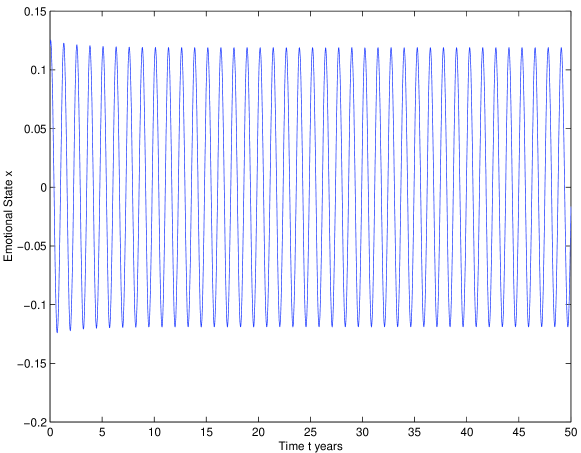
Figure 1: Time series representing the behavior of an untreated patient. The parameters are $\alpha=.36$, $\beta=-100$, and $\omega=5$. This leads to a stable limit cycle with an amplitude of about $.12$, which we designate as larger than that describing ‘normal’ mood swings.

Figure 2: Limit cycle corresponding to the time series in Figure 1. This describes the relationship between the individual’s moods and how fast they change.

Starting with the van der Pol oscillator caricature of the untreated patient, we apply the forcing function $g(x,\dot{x})$ to represent medication. We use (4) to represent a treated bipolar II patient, who possesses an unstable, large limit cycle (greater than the $.1$ amplitude, which is the threshold that we have chosen for ‘normal’ behavior) and a stable, small limit cycle. Choosing $\alpha=.1$, $\beta=-100$, and $\gamma=5000$ yields the plots in Figures 3 and 4.

Using the method of averaging,[23] we study the number and amplitude (denoted $A$) of the limit cycles of equation (4). The dynamics of $A$ are described by slow flow equations of motion, whose non-zero equilibria correspond to limit cycles of equation (4). Depending on the values of the parameters, there can be zero, one, or two limit cycles. The slow flow equations for the amplitude contain both positive and negative equilibria, but only the non-negative solutions are relevant to the original dynamical system. Limit-cycle amplitudes must satisfy

$$A^{2}=-\frac{\beta}{\gamma}\pm\frac{1}{\gamma}\sqrt{\beta^{2}-8\alpha\gamma}\,.$$ (6)

Once we find the limit cycle amplitudes, we compute the Jacobian (in this case, the second derivative) to determine their stability as functions of $\alpha$, $\beta$, and $\gamma$. There is always a slow-flow equilibrium at $A=0$, which corresponds to the equilibrium at $(0,0)$ of (4). We obtain the following conditions for the existence and stability of limit cycles:

1. Zero limit cycles occur when either $\beta^{2}-8\alpha\gamma<0$ (so that $A^{2}$ is not real) or $\alpha$, $\beta$, and $\gamma$ all have the same sign (so that $A^{2}<0$). In these cases, there are no slow-flow equilibria with positive $A$.

2. One limit cycle:

   • There is one limit cycle when $\beta/\gamma>0$ and $\beta^{2}=8\alpha\gamma$. There is a bifurcation at this point (corresponding to the coalescence of two limit cycles), and stability cannot be determined by computing a Jacobian.

   • There is one limit cycle when $\sqrt{\beta^{2}-8\alpha\gamma}>|\beta|$, regardless of the sign of $\beta/\gamma$. This occurs exactly when $\alpha\gamma<0$. Such a limit cycle is always unstable.

   • There is one limit cycle when $\alpha=0$ and $\beta/\gamma<0$. In this situation, the Jacobian is $-\beta^{2}/2\gamma$, so the limit cycle is stable if and only if $\gamma>0$.

3. Two limit cycles occur if $\beta/\gamma<0$ and $\beta^{2}>8\alpha\gamma>0$. This happens for $\gamma,\,\alpha>0$ when $\beta<0$ and for $\gamma,\,\alpha<0$ when $\beta>0$. In the biologically relevant situation describing a treated individual, the smaller limit cycle is stable. An example of this is depicted in Figures 3 and 4 with the parameter values $\alpha=.1$, $\beta=-100$, and $\gamma=5000$.

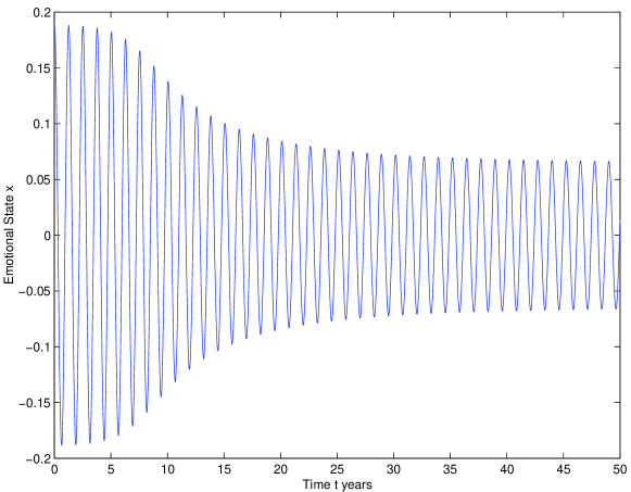
Figure 3: Treated patient with parameters $\alpha=.1$, $\beta=-100$, and $\gamma=5000$, which yields an unstable limit cycle with amplitude greater than $.1$ and a stable limit cycle with amplitude less than $.1.$ This patient begins to receive treatment at about age $5$ or $10$. Individuals usually first become bipolar between the ages of $18$ and $22$, but the onset of bipolar disorder can occur in early childhood.[7].

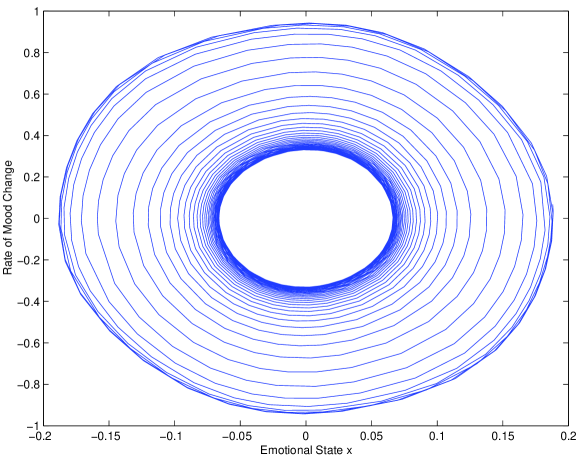
Figure 4: Limit cycles corresponding to the time series in Figure 3. The depicted trajectory approaches the smaller (stable) limit cycle as the time $t$ increases. The amplitude of this limit cycle is less than $0.1$, so it describes the mood swings of a functional individual.

3.2 Model 2: Liénard Oscillator with Autonomous Forcing

The introduction of a forcing function (representing treatment) to Model I results in smaller mood swings; in so doing, however, a larger unstable limit cycle was introduced. This has the potential drawback of predicting that if an individual goes too long without being diagnosed (and thus the amplitude of the mood swings is too large), one would need to ensure that the initial condition when treatment begins is within the basin of attraction of the smaller stable limit cycle. In other words, if the mood swings are too large, it might be necessary to drastically reduce the mood amplitude before introducing ‘normal’ treatment.

Model 2 provides an alternative minimalist framework to study bipolar II disorder that does not have this drawback. In this situation, we will demonstrate the presence of three limit cycles. We will also show that the ones with the largest and smallest amplitude are stable, whereas the limit cycle between them is unstable. Toward this end, we consider an equation of the form

$$\ddot{x}+f(x)\dot{x}+h(x)=g(x,\dot{x})\,,$$ (7)

where

$$g(x,\dot{x})=\rho\dot{x}^{3}+\mu\dot{x}^{5}+\nu\dot{x}^{11}\,.$$ (8)

For this model, we consider the constant function $f(x)=-0.38$ and the linear function $h(x)=180x$ together with the parameters $\mu=0.78$ and $\nu=-0.00093$. With $\rho=0.38$, we obtain a large stable limit cycle with mood amplitude approximately equal to $0.44$. As with Model 1, an untreated patient has bounded mood swings.

Without treatment, this model describes an individual with steadily worsening mood swings throughout his childhood and adolescent years. At approximately age $20$, the individual’s mood variations increase dramatically to the point where the individual can be clinically diagnosed with bipolar II disorder. For the given model and any initial conditions, the individual’s mood variations settle asymptotically to the stable limit cycle with mood swing amplitude $|x|\leq 0.45$, as shown in Figure 5. As this system’s limit cycle is globally stable, every trajectory eventually spirals toward it, yielding the time series depicted in Figure 6. Observe that the mood varies between $\pm 0.4465$. Moreover, the bipolar II individual described by this time series can diagnosed with both hypomania and severe depression at age 20.

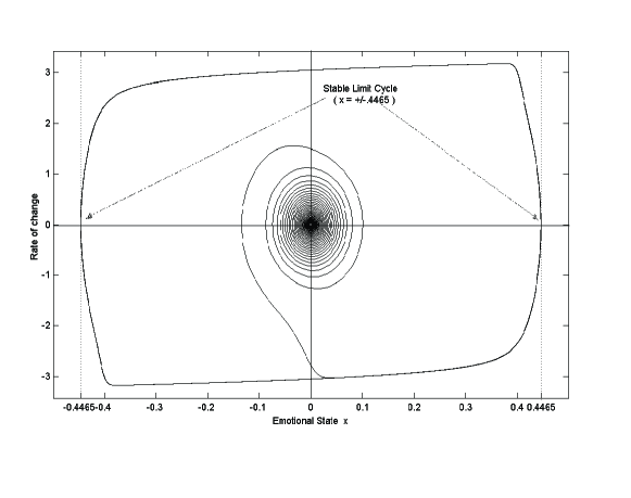
Figure 5: Untreated bipolar patient for Model 2. Only a large stable limit cycle is present.

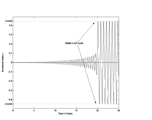
Figure 6: Time series corresponding to Figure 5. The initial condition lies inside the limit cycle and thus represents an individual who gradually worsens over time.

In considering the role of treatment $g(x,\dot{x})$ in this model, we note that $\rho$ is the key parameter that will be adjusted. For a treated patient, the value $\rho=-3.302$ (for example) yields qualitatively appropriate dynamics. A treated bipolar II patient is then modeled by

$$\ddot{x}-0.38\dot{x}+180x=-3.302\dot{x}^{3}+0.78\dot{x}^{5}-0.00093\dot{x}^{11}\,.$$ (9)

This model encompasses all aspects of treatment as a single function $g(x,\dot{x})$. In Figure 7, we see that by inputting the new initial conditions into the model that includes treatment, the patient exhibits favorable emotional patterns. There is a large stable limit cycle and an unstable limit cycle just inside it. A smaller stable limit cycle is the desired emotional pattern of the patient; all initial conditions lying inside the large unstable cycle yield solutions that spiral toward this smaller cycle, whose amplitude is sufficiently small so that the associated mood swings are deemed normal. One gets the same qualitative behavior with smaller $|\rho|$ (such as $|\rho|=2$), although the separation between the unstable limit cycle and the larger stable limit cycle surrounding it becomes larger as $|\rho|$ is decreased. The chosen value of $\rho$ yields limit cycles that are almost on top of each other; increasing $|\rho|$ destroys this qualitative structure.

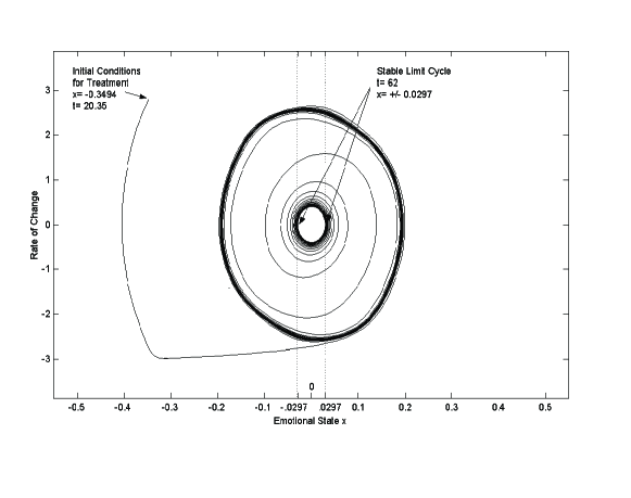
Figure 7: Treated bipolar II patient for Model 2. There is a large outer limit cycle which is stable and an unstable limit cycle lying just inside it. There is also a smaller stable limit cycle inside the unstable one; this orbit represents the desired mood swings of a treated patient.

The larger limit cycle prevents a treated patient from having unbounded mood variations that could otherwise occur, for example, if a perturbation were to make the current mood amplitude too large. The smaller stable limit cycle represents the desired low-amplitude mood variations. Comparing Figures 6 and 8 reveals that after treatment, the hypomanic and severe depressive episodes have both disappeared. At the beginning of treatment, the amplitude of the mood swings stays relatively close to $0.2$. It then tends asymptotically to the stable limit cycle, where the mood $x$ varies between approximately $\pm 0.03$. An important feature of the model demonstrated in Figure 7 is that treatment can begin at any time because the small limit cycle attracts all solutions that lie inside the unstable limit cycle. If the mood swings of the bipolar individual are initially too large, it may again be necessary for a brief drastic treatment to bring them into the basin of attraction of the smaller limit cycle before applying normal medication.

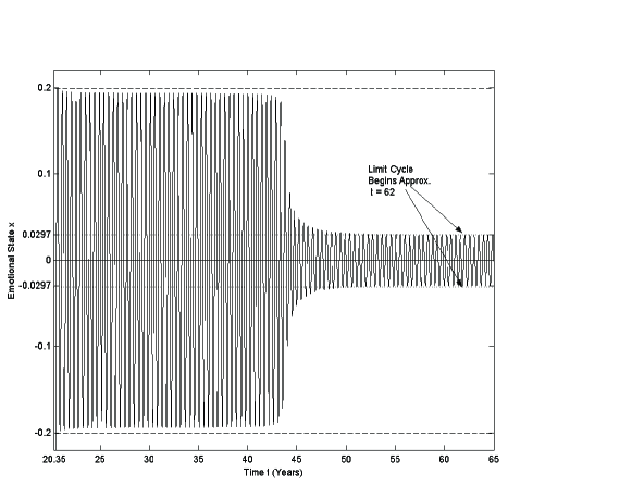
Figure 8: Time series corresponding to Figure 7. The initial condition lies inside the unstable limit cycle and is thus in the basin of attraction of the smaller stable limit cycle representing normal mood swings.

4 Bipolar Patients as Interacting Oscillators

Examining the possible effects two patients have on each other while undergoing treatment is of significant mathematical interest. Moreover, as mentioned previously, there are known cases of family units with multiple bipolar II individuals. Thus, the interaction of two bipolar patients is also of psychological interest.[29] It is known to occur, for example, in households with bipolar sibling pairs.[2] There has also been some work on using group treatment as a prophylaxis with patients in remission in order to prevent further episodes.[5] We again stress, however, that clinical data needs to be collected to examine these ideas more extensively.

Consider, for example, two treated bipolar II individuals, each of whom is separately described by equation (2). We transform into polar coordinates to provide a natural manner of adding coupling terms to represent the interaction between the two patients. Denoting by $K_{j}(r_{1},\theta_{1},r_{2},\theta_{2})$ the interactions between the patients, the dynamical system of interest is

$$\dot{r_{1}} =-\beta r_{1}^{3}(\cos{\theta_{1}})^{2}(\sin{\theta_{1}})^{2}$$

$$\quad+r_{1}\sin{\theta_{1}}{\left[\alpha\sin(\theta_{1})+\cos(\theta_{1})-\omega^{2}\cos(\theta_{1})\right]}+K_{1}(r_{1},\theta_{1},r_{2},\theta_{2})\,,$$

$$\dot{\theta_{1}} =\alpha\sin(\theta_{1})\cos(\theta_{1})-(\sin{\theta_{1}})^{2}$$

$$\quad-\omega^{2}(\cos{\theta_{1}})^{2}-\beta r_{1}^{2}(\cos{\theta_{1}})^{3}\sin(\theta_{1})+K_{2}(r_{1},\theta_{1},r_{2},\theta_{2})\,,$$

$$\dot{r_{2}} =-\beta r_{2}^{3}\cos{\theta_{2}}^{2}(\sin{\theta_{2}})^{2}$$

$$\quad+r_{2}\sin{\theta_{2}}{\left[\alpha\sin(\theta_{2})+\cos(\theta_{2})-\omega^{2}\cos(\theta_{2})\right]}+K_{3}(r_{1},\theta_{1},r_{2},\theta_{2})\,,$$

$$\dot{\theta_{2}} =\alpha\sin(\theta_{2})\cos(\theta_{2})-(\sin{\theta_{2}})^{2}$$

$$\quad-\omega^{2}(\cos{\theta_{2}})^{2}-\beta r_{2}^{2}(\cos{\theta_{2}})^{3}\sin(\theta_{2})+K_{4}(r_{1},\theta_{1},r_{2},\theta_{2})\,.$$ (10)

For simplicity, we assume that the phase difference affects only the phase terms and the amplitude difference affects only the amplitude terms. We also assume linear proportionality, so that the coupling terms simplify to

$$K_{1} =k_{1}(r_{2}-r_{1})\,,\quad K_{2}=k_{2}(\theta_{2}-\theta_{1})\,,$$

$$K_{3} =k_{3}(r_{1}-r_{2})\,,\quad K_{4}=k_{4}(\theta_{1}-\theta_{2})\,,$$ (11)

where the $k_{i}$ are the proportionality constants. An important detail to note is that the angular coupling terms in (11) include no limitation on the phase angle, so that $\theta_{1}-\theta_{2}$ can increase beyond $2\pi$. There is no difficulty, however, when we convert back to rectangular coordinates. The coupling terms remain bounded, as the radial coupling terms are proportional to $\sqrt{x_{i}^{2}+\dot{x}_{i}^{2}}$ and the angular ones are proportional to $\arctan(\dot{x}/x)$. When we numerically integrate these dynamical equations, we utilize $\arctan\,(\dot{x}/x)\in(-\pi/2,\pi/2)$. Although the arctangents in rectangular coordinates create a discontinuous vector field, the behavior near the discontinuities correctly models the biology observed in situations in which two patients with bipolar disorder are interacting. (That is, we observe fluctuations near in-phase and out-of-phase modes).

Other choices of coupling terms avoid unbounded phase differences. Consider, for example,

$$K_{1} =k_{1}(r_{2}-r_{1})\,,\quad K_{2}=k_{2}\sin(\theta_{2}-\theta_{1})\,,$$

$$K_{3} =k_{3}(r_{1}-r_{2})\,,\quad K_{4}=k_{4}\sin(\theta_{1}-\theta_{2})\,,$$ (12)

where the $k_{i}$ are again proportionality constants. We have conducted some mathematical analysis of (10) with both (11) and (12) and discuss one of our results briefly. Note, however, that although these results are mathematically interesting, we only mention these models in passing because insufficient clinical data is available to properly constrain the numerous forms of coupling available when constructing mathematical models describing interacting bipolar II individuals. Consequently, we only state results for two common types of solutions in such systems.

In coupled systems, important types of behavior include in-phase modes, for which $x_{1}=x_{2}$ and $y_{1}=y_{2}$, and out-of-phase modes, for which $x_{1}=-x_{2}$ and $y_{1}=-y_{2}$. For the first form of coupling (11), both in-phase and out-of-phase modes exist and are stable with relatively small basins of attractions. Larger stable motions exist that attract initial conditions starting outside those basins of attraction. Both in-phase and out-of-phase modes also exist with the second form of coupling (12), and the former appears to be the only stable motion in the system. Initial conditions starting far away from the in-phase mode eventually approach this mode.

Interpreted biologically, two coupled bipolar II individuals with similar moods ($x_{1}\approx x_{2}$) and mood cycling rates ($y_{1}\approx y_{2}$) tend to remain in-phase. They are synchronized in the sense that they enter hypomanic and depressive states (roughly) concurrently. The same argument applies to out-of-phase modes, so if two bipolar II individuals are almost completely out-of-phase, they will remain that way. One individual enters a hypomanic phase when the other enters a depressive phase.

5 Discussion

In this work, we proposed two limit cycle oscillator models that attempt to explain qualitatively the moods swings of bipolar II individuals. There is insufficient data at this time to construct a quantitatively detailed model describing bipolar disorder, so this first step employing minimalist models is an essential one. Indeed, similar phenomenological models have yielded significant insight into the dynamics of several oscillatory biological and physical phenomena.[3, 4, 30]

Even without time-series data to describe the moods of bipolar patients, the models we have developed could prove important in increasing the understanding of the effect of treatment on the cyclic behavior of bipolar individuals. Because the two-dimensional dynamical systems we utilize provide simple caricatures of the behavior of bipolar individuals, it is concomitantly easy to analyze these models. Moreover, despite their simplicity, they successfully capture qualitatively the known behavior of treated and untreated bipolar II individuals. A quantitative analysis of their dynamics, which is our long-term goal, will require refining our models using time-series data from clinical trials. It is our hope that the present work will stimulate further mathematical treatments that incorporate such data as well as the data collection that will permit these modeling efforts.

In Model 1, we considered treatment as a forcing function that led to a stable limit cycle with smaller amplitude, which we interpreted as a decrease in the severity of the mood swings of the bipolar patient. This model suggests that individuals that are not diagnosed at a sufficiently young age might need drastic intervention to bring their mood swings to a reasonable level. Given that individuals are usually diagnosed in the depressive state and that bipolar disorder is frequently misdiagnosed initially, this aspect of Model 1 is especially noteworthy.[19, 8]

Model 2 provides an alternative framework in which a bipolar II individual possesses two stable limit cycles even without treatment; satisfactory treatment then confines the patient to the one with smaller amplitude. The rapid cycling induced by Desiramine Hydrochloride that was reported by Wehr and Goodwin[28] can be interpreted as a slight increase in the amplitude of the oscillation but—more centrally—as an increase in the oscillation frequency. This phenomenon can be addressed within the modeling framework we have developed by allowing the frequency parameter to also be perturbed slightly by treatment.

At this point, it is also important to briefly consider how our models can be both refined and generalized. First, incorporating biological data is of paramount importance. We used minimal data because little data is available in a form that facilitates the creation or refinement of mathematical models. This is the largest deficiency in our analysis; employing our modeling framework along with data from psychological testing of bipolar II individuals will yield a significantly increased understanding of this medical condition. In fact, one of the primary purposes of this work is to motivate the collection of such data so that detailed models of bipolar disorder can ultimately be developed. In addition to time-series data describing the behavior of a large number of bipolar patients, it is also desirable to have data describing the mood variations of “normal” individuals to provide a basis for comparison.

Numerous generalizations of our models can be considered to further examine mood disorders using limit-cycle oscillators. For example, one can incorporate the fact that the medication administered to bipolar II individuals typically take several days to reach therapeutic levels in the blood stream by adding a time-delay to the treatment function. One can also gain further mathematical and biological insight by directly examining the bifurcations that occur in our models. Moreover, one can incorporate explicit time-dependence (for example, via delta functions representing instantaneous medication) into the treatment function by considering a nonautonomous forcing function $g(x,t)$.

Limit cycle oscillators can also be used to study behavioral cycling in mood disorders besides bipolar disorder, as such phenomena are of considerable interest to both psychologists and psychiatrists.[8] Pertinent disorders include unipolar depression and cyclothymia. Individuals suffering from the latter disorder rapidly flip back and forth between depressed and euphoric moods. Their high and low periods, which are relatively short, are much less intense than those of bipolar individuals. Although it is not known precisely what leads individuals from one pole to the other, possible causes include psychosocial stress, disrupted sleep patterns, or some endogenous or internal biological mechanism that is not connected to environmental stimuli.[24] It is also not known what happens to cycling over time. It is speculated that an individual’s cycling may slow down with age. From a mathematical perspective, we wish to highlight that the effects of disrupted sleep patterns can be studied by coupling a cyclothymic (or bipolar) individual with a limit-cycle oscillator representing the human sleep-wake cycle.[26]

Another important issue to consider is the threshold for flipping poles. It has been theorized, for example, that the threshold for depression (and for flipping poles) gets lower over time. It has been speculated (by Robert Post[21], for example) that the longer one is ill, the more autonomous or disconnected episodes become from the environment. This is termed “kindling theory” and is believed to be analogous to what happens in epilepsy, in which there is a gradual kindling of biological disturbances in the brain that eventually surpasses the threshold for a seizure.

6 Conclusions

In this paper, we provide a mathematical framework for the modeling of bipolar disorder in terms of low-dimensional limit cycle oscillators. We propose and analyze two phenomenological models of bipolar individuals. Rather than focusing on the method of diagnosis, which is a difficult medical problem, we instead concentrate on the dynamics of our models under the proposed treatment strategy, which involves a combination of drugs and therapy. The purpose of our modeling efforts is not to suggest a specific treatment for bipolar individuals but rather to provide some insight into the complicated dynamics of bipolar disorder. In this respect, we view our work as a first step in developing mathematical models of the mood swings of bipolar individuals. Our intent is to provide a mathematical framework that ultimately leads to the development of more detailed models of bipolar disorder that incorporate clinical data. With this work, we hope to motivate the collection of time-series data from clinical trials that will lead to refinements of our model that incorporate such data. In our view, dynamical systems theory and mathematical modeling in general can lead to important advancements in the understanding of bipolar disorder.

References

- [1] American Psychiatric Association (2000), Diagnostic and statistical manual of mental disorders : DSM-IV-TR. American Psychiatric Association, Washington DC.
- [2] P. Bennett, R. Segurado, et al. (2002), The Wellcome trust UK-Irish bipolar affective disorder sibling-pair genome screen: first stage report. Molecular Psychiatry, 7: 2, 189-200.
- [3] Erika T. Camacho (2003), Mathematical Models of Retinal Dynamics Ph.D. Thesis, Center for Applied Mathematics. Cornell University, Ithaca, NY.
- [4] Erika T. Camacho, Richard H. Rand, and Howard H. Howland (2004) Dynamics of Two van der Pol Oscillators Coupled via a Bath Special Boley Issue of the International Journal of Solids and Structures, 2004.
- [5] Francesco Colom, Eduard Vieta, el al. (2003), A randomized trial on the efficacy of group psychoeducation in the prophylaxis of recurrences in bipolar patients whose disease is in remission. Archives of General Psychiatry, 60: 4, 402-407.
- [6] Cindy L. Ehlers (1995), Chaos and complexity: Can it help us to understand mood and behavior? Arch Gen Psych, 52: 960-964.
- [7] Jan Fawcett, M.D., Bernard Golden, Ph.D., and Nancy Rosenfeld (2000), New Hope for People with Bipolar Disorder, Prima Publishing, Roseville, CA.
- [8] I. Nicol Ferrier, Iain C. Macmillan, and Allan H. Young (2001), The search for the wandering thymostat: a review of some developments in bipolar disorder research, British Journal of Psychiatry, 178: 41, s103-s106.
- [9] Paula Ford-Martin (1995), Bipolar Disorder. Gale Encyclopedia of Alternative Medicine, January 01.
- [10] Ellen Frank, Holly A. Swartz, and David J. Kupfer (2000), Interpersonal and Social Rhythm Therapy: Managing the Chaos of Bipolar Disorder. Biological Psychiatry, 48: 6, 593-604.
- [11] Hector Giacomini and Sebastian Neukirch (1997), On the Number of Limit Cycles of the Liénard Equation. Physical Review E, 56: 4.
- [12] Stephen W. Good (2000), Differential Equations and Linear Algebra, second edition. Prentice-Hall Inc. Upper Saddle River, New Jersey, Second Edition.
- [13] A. Gottschalk, M. S. Bauer, and P.C. Whybrow (1995), Evidence of chaotic mood variation in bipolar disorder, Arch Gen Psychiatry, 52: 947-959.
- [14] Kim Griswold (2000), Management of Bipolar Disorder. American Family Physician, September 15.
- [15] J. Guckenheimer, M. Meyers, F. Wicklin, and P. Worfolk (1991), DSTool: Dynamical System Toolkit with an Interactive Graphical Interface. Department of Applied Mathematics, Cornell University, Ithaca, NY.
- [16] David Haslam, MSc, MD, Sidney Kennedy, MD, FRCPC, Vivek Kusumakar, MD, FRCPC, Stan Kutcher, MD, FRCPC, Raymond Matte, MD, FRCPC, Sagar Parikh, MD, FRCPC, Peter Silverstone, MD, FRCPC, Verinder Sharma, MBBS, FRCPC, Lakshmi Yatham, MD, FRCPC, A Summary of Clinical Issues and Treatment Options. Bipolar Disorder Sub-Committee Canadian Network for Mood and Anxiety Treatments (CANMAT). http://www.canmat.org/gpsfps/nine/bipolar.html.
- [17] Lewis L. Judd, Hagop S. Akiskal, et al. (2003), A Prospective Investigation of the Natural History of the Long-term Weekly Symptomatic Status of Bipolar II Disorder Archives of General Psychiatry, 60: 3, 261-269.
- [18] Terry Kupers (June 29, 2002), Private Communication, Wright Institute.
- [19] L. Lewis and L.A. Vornik (2003), Perceptions and impact of bipolar disorder: How far have we really come? Results of the National Depressive and Manic Depressive Association 2000 survey of individuals with bipolar disorder, Journal of Clinical Psychiatry, 64: 2, 161-174.
- [20] Iain C. Macmillan (May 25, 2004), Private Communication, Consultant Psychiatrist, Early Intervention Service, Norfolk Mental Health Care NHS Trust.
- [21] Robert M. Post (1992), Transduction of psychosocial stress into the neurobiology of recurrent affective disorder, American Journal of Psychiatry, 149, 999-1010.
- [22] Robert M. Post and David A. Luckenbaugh (2003), Unique design issues in clinical trials of patients with bipolar affective disorder, Journal of Psychiatric Research, 37: 1, 61-73.
- [23] Richard H. Rand (1994), Topics in Nonlinear Dynamics with Computer Algebra, Computation in Education: Mathematics, Science and Engineering Series, vol. 1, Gordon and Breach Science Publishers, USA.
- [24] Lawrence Riso (July 9, 2003), Private Communication, Department of Psychology, Georgia State University.
- [25] Steven H. Strogatz (1994), Nonlinear Dynamics and Chaos: With Applications in Physics, Biology, Chemistry, and Engineering. Reading, Mass: Addison-Wesley Publishing Company.
- [26] Steven H. Strogatz (1986), The Mathematical Structure of the Human Sleep-Wake Cycle. Lecture Notes in Biomath. 69. New York, NY: Springer-Verlag.
- [27] Peter Totterdell, Rob B. Briner, Brian Parkinson, and Shirley Reynolds (1996) Fingerprinting time series: Dynamic patterns in self-report and performance measures uncovered by a graphical non-linear method. British Journal of Psychology, 87: 43-60.
- [28] Thomas A. Wehr and Frederick K. Goodwin (1979), Rapid Cycling in Manic-Depressives Induced by Tricyclic Antidepressants. Arch Gen Psychiatry, 36: 555-559.
- [29] Roger D. Weiss, Margaret L. Griffin, et al. (2000), Group therapy for patients with bipolar disorder and substance dependence: Results of a pilot study. Journal of Clinical Psychiatry, 61: 5, 361-367.
- [30] Stephen A. Wirkus and Richard H. Rand (2002), The Dynamics of Two Coupled van der Pol Oscillators with Delay Coupling, Nonlinear Dynamics, 30: 3, 205-221.