Extreme waves and modulational instability: wave flume experiments on irregular waves

Abstract

We discuss the formation of large amplitude waves for sea states characterized by JONSWAP spectra with random phases. In this context we discuss experimental results performed in one of the largest wave tank facilities in the world. We present experimental evidence that the tail of the cumulative probability function of the wave heights for random waves strongly depends on the ratio between the wave steepness and the spectral bandwidth. When this ratio, called the Benjamin-Feir Index, is large the Rayleigh distribution clearly underestimates the occurrence of large amplitude waves. Our experimental results are also successfully compared with previously performed numerical simulations of the Dysthe equation.

I Introduction

The determination of the probability density function of wave heights for a system of a large number of random waves is definitely a task of major importance both from theoretical and applicative points of view. For linear waves the fundamental work was done by Rice (1944) in connection with noise in electronic circuits. Some years later Longuet-Higgins (1952) adapted the ideas of Rice to surface gravity waves. He showed that if the wave spectrum is narrow banded and if the phases of the Fourier components of the surface elevation are distributed uniformly (random phases), then the probability distribution of crest-to-trough wave heights is given by the Rayleigh distribution. In the study of extreme events, it is useful to define the probability that the wave height $H$ assumes a value greater than a reference height, $H_{0}$. This probability, also known as the survival function $S(H>H_{0})$, is given by $1-P(H\leq H_{0})$, where $P$ is the cumulative probability function. For the Rayleigh distribution the survival function is given by:

$$S(\xi>\xi_{0})=Exp[-2\xi_{0}^{2}],$$ (1)

where $\xi=H/H_{s}$, with $H_{s}$ the significant wave height. Using the survival function, it is for example possible to establish that the probability of finding a wave whose height is greater than two times the significant wave height is about 1/2980. The value of two is usually selected as a threshold for identifying abnormally high waves (also known as freak waves) in a surface elevation time series.

After the pioneering work by Longuet-Higgins (1952), the validity of the Rayleigh distribution for wave heights has been widely investigated. The distribution (1) was found to agree well with many field observations (Earle, (1975)) even though the frequency spectrum was not always so narrow and the steepness was not as small as required by the theory. During the last 30 years, many empirical distribution functions have been proposed to fit better the data. Forristall (1978) analyzed data recorded during hurricanes in the Gulf of Mexico and obtained a better agreement with a two parameter Weibull distribution. According to his analysis, the Rayleigh distribution was over-predicting the experimental data. Some years later Longuet-Higgins (1980) re-examined the same data and showed that the Rayleigh distribution fitted equally well the data, provided that the value of the root mean square of the amplitude is suitably modified by introducing a finite spectral band width (see also Naess (1985)).

In recent years particular attention has been given to understanding the mechanism of formation of freak waves and their influence on the tail of the probability density function of wave heights. Even though a number of physical mechanisms have been identified (linear superposition, Longuet-Higgins (1952), the wave-current interaction, see Lavrenov (1998) and White and Fornberg (1998), and the modulational instability, see Henderson et al. (1999), Trulsen and Dysthe (1997),Tulin and Waseda (1999)), it should be stated that not much theoretical progress has been made concerning the resulting statistical properties of the surface elevation. More in particular, the relation between the various sea states and the probability density function has not been clearly identified.

Limiting the study to one-dimensional propagation, Onorato et al. (2000) have performed numerical simulations of the Nonlinear Schroedinger and Dysthe equations with initial conditions provided by the random JONSWAP spectrum with different values of the enhancement factor $\gamma$ and the Phillips constant $\alpha$ ($\gamma$ is related to the spectral band-width and the wave steepness; $\alpha$ is responsible for the energy content of the surface elevation and therefore contributes to the wave steepness). One interesting result obtained is that the probability density function drastically depends on these two parameters $\alpha$ and $\gamma$. For small values of $\alpha$ and $\gamma$ the Rayleigh distribution approximates the data rather well, but for large values of $\alpha$ and $\gamma$ the Rayleigh distribution clearly under estimates the tail of the probability density function (see Figure 6b in Onorato et al. (2000)). For example, using the Dysthe equation, with a JONSWAP spectrum with $\gamma=6$ and $\alpha=0.0081$ as initial condition, the probability of recording a freak wave (defined as a wave whose height is at least two times the corresponding significant wave height) is 1/630, almost 5 times greater than the one predicted by the Rayleigh distribution! Strong departure from the Rayleigh distribution was also observed numerically by Mori and Yasuda (2000) and by Brandini (2001), using the Higher Order Spectral method of Dommermuth and Yue (1987) for solving the Euler equations for surface gravity waves. This departure from the Rayleigh distribution was attributed to the Benjamin-Feir instability mechanism that, provided the spectrum is sufficiently narrow and the steepness is sufficiently large, can take place also in random waves (Alber (2000)).

Following the ideas developed in Alber (2000) and successively in Janssen (1991), Onorato et al. (2003) studied the instability of a narrow banded approximation of a JONSWAP spectrum, individuating the region of instability of the spectrum in the $\alpha$-$\gamma$ plane. They found that from random spectra, as a result of the modulational instability, oscillating coherent structures may be excited (these structures are particular “breather” solutions of the NLS equation Dysthe and Trulsen (1999), Osborne et al. (2000)). More recently Janssen (2003) discovered that the region of instability predicted using the theory developed in Alber (2000) is not completely consistent with direct simulations of the NLS and Zakharov equations. He therefore developed a kinetic equation that takes into account quasi-resonant interactions and demonstrated good agreement between theory and direct numerical simulations; moreover he was also able to compute from the theory some statistical properties of the surface elevation such as for example the kurtosis. He found out that, if the ratio between the steepness and the spectral bandwidth is large (the ratio is often referred to as the Benjamin-Feir Index (BFI), see also Onorato et al. (2001)), the gaussian distribution underestimates the tails of the probability density function for the surface elevation. Note that in his analysis the statistics was computed only on free waves, the Stokes contribution was not included. Even though it was not mentioned in the paper, we expect that in such conditions also the survival function for wave heights should be far from being well described by (1). One of the major results in Janssen (2003), that confirms previous results from numerical simulations in Onorato et al. (2000) and Onorato et al. (2001), is therefore that the statistical properties of the surface elevation strongly depend on the BFI and therefore on the spectral shape (see section II). This conclusion, limited to deep water waves and to one dimensional propagation, has been reached from simplified models, without including any mechanism of dissipation such as wave breaking.

Concerning random wave experiments in wave tank facilities, in the past 15 years it has been recognized that at about 15-20 wave-lengths from the wave maker extreme individual wave heights in random records may appear more frequently than predicted by the Rayleigh distribution (see for example Stansberg (2000) and references therein). The increase of the kurtosis observed along the wave tank in Stansberg (1992) was interpreted as a higher-order effect, attributed to the modulational instability. Nevertheless, to the knowledge of the authors, even though JONSWAP spectra are the most common runs in wave flumes for many different applications, there has not been any systematic experimental study devoted to understanding the relation between the BFI and probability density function of wave heights.

In this paper we discuss some interesting experimental results that we have obtained in a large facility at Marintek, Trondheim (Norway). Our main goal in this paper is to give some experimental support to the numerical and theoretical work performed in recent years that suggests the idea that the modulational instability can be responsible for the formation of freak waves. Our experimental results, compared successfully with previously performed numerical simulations of the Dysthe equation, show that the probability density function of wave heights depends strongly on the BFI. The paper is organized as follows: Section II contains a derivation of the BFI; with respect to previous work we extend the definition of the BFI to arbitrary depth. Sections III and IV are devoted to the description of the experiment and of the results. Discussions and conclusions are reported in section V.

II The Benjamin-Feir Index and its relation to the JONSWAP spectrum

The Benjamin-Feir Index has been introduced formally in the paper by Janssen (2003) and can be obtained in two different ways. The first more laborious one consists in following the approach by Alber (2000), i.e. one starts from the Nonlinear Schroedinger equation, derives a kinetic equation for inhomogeneous surface elevation, performs a linear stability analysis of an homogeneous random spectrum and obtains its condition of stability (see Janssen (2003) for details). The resulting condition simply states that a spectrum is stable if the BFI is less than one. A simpler approach, the one that will be presented here, proposed in Onorato et al. (2001), is based on dimensional arguments (note that in Onorato et al. (2001) the square of the BFI was considered and was referred to as an Ursell number). Consider the dimensional NLS equation in arbitrary depth, in a frame of reference moving with the group velocity:

$$\frac{\partial A}{\partial t}+i\sigma\frac{1}{8}\frac{\omega_{0}}{k_{0}^{2}}\frac{\partial^{2}A}{\partial x^{2}}+i\beta\frac{1}{2}\omega_{0}k_{0}^{2}|A|^{2}A=0,$$ (2)

where $A$ is the complex wave envelope, $k_{0}$ is the carrier wave number corresponding and $\omega_{0}$ is the respective angular frequency. $\sigma$ and $\beta$ are functions of the product $k_{0}h$, with $h$ the water depth, and both tend to 1 as $k_{0}h\rightarrow\infty$. The analytical form of $\sigma$ and $\beta$ can be found for example in the book of Mei (1983). The next step consists in adimensionalizing equation (2) in the following way: $A^{\prime}=A/a_{0}$, $x^{\prime}=x\Delta K$ and $t^{\prime}=t(\Delta K/k_{0})^{2}\sigma\omega_{0}/8$, where $\Delta K$ represent a typical spectral bandwidth, $a_{0}$ a typical wave amplitude. Equation (2) reduces to:

$$\frac{\partial A}{\partial t}+i\frac{\partial^{2}A}{\partial x^{2}}+i\bigg{(}\frac{2\epsilon}{\Delta K/k_{0}}\bigg{)}^{2}\frac{\beta}{\sigma}|A|^{2}A=0,$$ (3)

where primes have been omitted. $\epsilon=a_{0}k_{0}$ is a measure of the wave steepness. We define the Benjamin-Feir Index as the square root of the coefficient that multiplies the nonlinear term (a factor of $2/\sqrt{2}$ is included to recover the definition in Alber (2000)):

$$BFI=\frac{{\sqrt{2}}\epsilon}{\Delta K/k_{0}}\sqrt{\frac{\beta}{\sigma}}$$ (4)

The definition corresponds to the one in Janssen (2003), except for the term $\sqrt{{\beta}/{\sigma}}$ on the right hand side which we have included here to include the influence of the water depth. The effect of this last term on the BFI as a function of $k_{0}h$ is shown in Figure 1. As the water depth increases the function tends to one and goes to zero for shallower water. For values of $k_{0}h$ smaller than about 1.36, the BFI looses its meaning because, as it is well known, the coefficient in front of the nonlinear term in the NLS changes sign and the equation becomes stable with respect to side band perturbations. As the BFI index increases the nonlinearity increases; therefore we expect that the number of freak waves increases. Note that this result was first obtained numerically with numerical simulations of the NLS equation in Onorato et al. (2001).

Normally one measures time series rather than space series; therefore, for the computation of the BFI from experimental data, the term in the BFI for infinite water depth $\Delta K/k_{0}$ should be replaced by $2\Delta f/f_{0}$ where $f_{0}$ is the frequency at the spectral peak and $\Delta f$ spectral-band width. Therefore, given a time series, we estimate the BFI in the following way: the wave spectrum is computed; the spectral half-width at half maximum provides an estimate of the spectral-band width, $\Delta f$. Methods such as those based on the quality factor (see for example Janssen (1991)) could also be used for the calculation of the spectral width. Nevertheless for our purposes, we find our simple and straightforward method to be satisfactory. Using the linear dispersion relation, the peak frequency is converted into the peak wave-number and the steepness is then computed as $\epsilon=k_{0}H_{s}/2$, where $H_{s}$ is the significant wave height computed as 4 times the standard deviation of the time series.

Figure 1: Effect of finite water depth on the BFI

We have applied this methodology in order to establish the relation between the BFI and the JONSWAP spectrum, see Komen et al. (1994):

$${P(f)=\frac{\alpha g^{2}}{(2\pi)^{4}f^{5}}\exp\bigg{[}-\frac{5}{4}\bigg{(}\frac{f_{0}}{f}\bigg{)}^{4}\bigg{]}\gamma^{\exp[-\frac{(f-f_{0})^{2}}{2\sigma_{0}^{2}f_{0}^{2}}]},}$$ (5)

where $\sigma_{0}$=0.07 if $f\leq f_{0}$ and $\sigma_{0}$=0.09 if $f>f_{0}$, $g$ is gravity acceleration, $\alpha$ is the Phillips constant and $\gamma$ is the enhancement parameter. In Figure 2 we show the BFI as a function of the $\gamma$ for $\alpha=0.01$ and $\alpha=0.02$ (here we have considered the case of infinite water depth. We note that for $\alpha$ fixed, larger values of $\gamma$ imply a larger value of the Benjami-Feir-Index. The Phillips constant $\alpha$ is strictly related to the wave energy, therefore to the wave steepness, $\alpha\sim\epsilon^{2}$. If we double the value of $\alpha$ with $\gamma$ fixed the steepness increase by a factor of $\sqrt{2}$ and so does the BFI (the spectral band-width remains practically unchanged.)

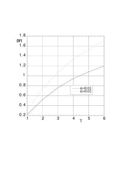
Figure 2: BFI as a function of the enhancement parameter $\gamma$ for $\alpha=0.01$ and $\alpha=0.02$

III Description of the experiments

The experiment was carried out in the long wave flume at Marintek (see Stansberg (1993) for details). The length of the tank is $270$ $m$ and its width is $10.5$ $m$. The depth of the tank is 10 meters for the first 85 meters and then is reduced to 5 meters for the rest of the flume. The effect of the jump from 10 to 5 meters is insignificant for the waves of 1.5 seconds considered here: It can be easily seen from linear theory that the particle velocities at 5 meter depth are essentially zero. A horizontally double-hinged flap type wave-maker located at one end of the tank was used to generate the waves. The distribution of signal frequencies to the upper and lower flap is automatically made by control software. All flap motion is computer controlled by using pre-generated digital control signals stored in files. A sloping beach is located at the far end of the tank opposite the wave maker. After half an hour of an irregular wave run with peak period of 1.5 seconds, the wave reflection was estimated to be less than 5%. The wave surface elevation was measured simultaneously by 19 probes placed at different locations along the flume (Figure 3). Twin-wire conductance measuring probes were used; these have excellent calibraion characteristics. Each wire was $0.3$ $mm$ in diameter, separated $10$ $mm$ from its twin in the direction perpendicular to the main axis of the tank. A schematic of the flume with the location of the probes is shown in Figure 3. Preliminary simulations with the one dimensional NLS equation were performed in order to estimate the spatial scales needed for the modulational instability to develop in a random spectrum. Note that an estimation of these scales based on the dispersion relation from small perturbation theory of plane solutions is not adequate because in a random JONSWAP spectrum the perturbations are never small! For steepness of around 0.1, we estimated from numerical simulations that the instability would take place at around 20-25 wavelengths, i.e for 1.5 seconds waves at around 60-75 meters from the wave maker. This is why a larger number of probes were placed in that region. Lateral probes were also placed at 75 and 160 meters in order to verify the quality of the long-crested waves generated at the wave maker. The sampling frequency for each probe was 40 Hz.

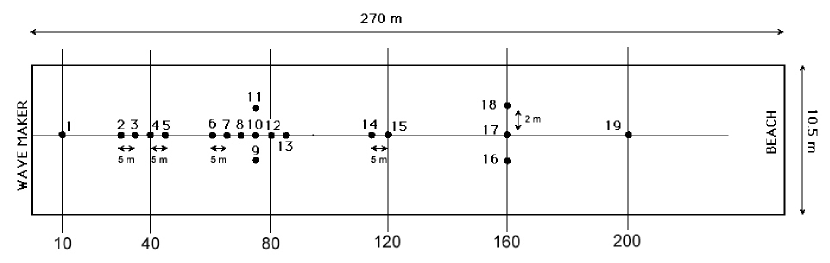
Figure 3: Schematic of the wave tank facility at Marintek and location of wave probes.

JONSWAP random wave signals where synthesized as sums of independent harmonic components, by means of the inverse Fast Fourier Transform of complex random Fourier amplitudes. These were prepared according to the “random realization approach” by using random spectral amplitudes as well as random phases. Three different JONSWAP spectra with different values of $\alpha$ and $\gamma$ have been investigated. All of them were characterized by a peak period of 1.5 seconds. In Table 1 we report the parameters that characterized each JONSWAP spectrum. The three different experiments will be called BFI0.2, BFI0.9 and BFI1.2, with obvious meaning. The value of $\sqrt{\beta/\sigma}$ in the BFI was estimated to be 0.95 at the wave maker.

$\gamma$	$H_{s}(m)$	$\epsilon=k_{0}H_{s}/2$	$\Delta f/f_{0}$	BFI
1	0.11	0.098	0.28	0.2
3.3	0.14	0.125	0.09	0.9
6	0.16	0.142	0.08	1.2

Table 1: Parameters of the three different experiments performed at Marintek

In order to have sufficiently good statistics, a large number of waves was recorded. Note that the large amount of data is of fundamental importance for the convergence of the tail of the probability density function for wave heights. Therefore for each type of spectrum, 5 different realizations with different sets of random phases have been performed. The duration of each realization was 32 minutes. The total number of wave heights (counting both up-crossing and down-crossing) recorded for each spectral shape at each probe was about 12800 waves. In our analysis we have removed the first 200 seconds of the records for each realization. This lapse of time was calculated as the approximate time needed for the wave of frequency corresponding to twice the peak-frequency to reach the last probe.

IV Experimental Results

We first study the behavior of some statistical quantities that can give an indication on the presence of extreme events in the time series. In particular we consider the fourth-order moment of the probability density function, the kurtosis, that gives an indication of the importance of the tail of the distribution function. We recall that for a Gaussian distribution the value of the kurtosis is 3, while larger values of kurtosis in a measured time series can give an indication of the presence of extreme events. In Figure 4 we show the kurtosis for the three experiments as a function of the distance from the wave-maker. The axes has been adimensionalized using the wave-length corresponding to the peak period at the wave-maker: for $T$=1.5 seconds, $L$=3.51 meters. First of all it should be noted from the Figure that the kurtosis is always greater than the Gaussian prediction. For larger BFI (BFI=0.9 and BFI=1.2) the kurtosis grows very fast and reaches its maximum between 25 and 30 wave lengths from the wave maker. This result is qualitatively consistent with our preliminary numerical analysis conducted with the NLS equation from which it was estimated that the typical space scale of the modulational instability was of the order of 20-25 wave lengths. After 30 wave-lengths from the wave-maker the kurtosis decreases. This behavior could be due to a reduction of the modulational instability activity because of the reduction of the wave steepness: waves have lost some energy due to wave-breaking (visible during experiments); moreover downshifting of the peak period also takes place. Locally, especially when the steepness is very large, three dimensional effects could also take place Trulsen et al. (1999). For the smallest value of the BFI considered, it is shown that the kurtosis is almost constant with a mean value of 3.19. This result suggests a significant dependence on the BFI of the statistical properties of surface gravity waves. From Figure 4 we expect to find a larger number of extreme events for larger values of the BFI. It should be mentioned that similar results as those obtained for the BFI0.9 have been obtained previously in Stansberg (2000), carried out with approximately the same BFI, but in shorter and much wider basin (50 m x 80 m). This indicates quite well that observed effects are independent of the facility used in the experiment.

Figure 4: Evolution of the kurtosis along the wave tank: BFI0.2, crosses; BFI0.9, empty circles; BFI1.2 full circles (see Table 1). The horizontal axis has been non-dimensionalized with the characteristic wavelength computed using the linear dispersion relation.

We then turn our attention to wave heights and define from a time series the density of rogue waves as the number of wave heights, considering both zero up-crossing plus down-crossing waves, that satisfies the conditions $H\geq 2H_{s}$ over the total number of wave heights recorded. In Figure 5 we show the rogue wave density for each probe at different distances from the wave maker. Up to around 15 wavelengths from the wave maker the rogue wave density is bounded between $10^{-4}$ and $10^{-3}$. While the density for BFI0.2 remains more or less at the same level, the rogue wave density increases substantially for BFI0.9 and BFI1.2 reaching a maximum of $3.1$x$10^{-3}$ for BFI1.2. Then in the last part of the tank the number of rogue waves decreases. This result is consistent with the analysis of the kurtosis previously presented. According to our expectations, the number of rogue waves recorded increases as the Benjamin-Feir Index of the initial condition increases.

Figure 5: Rogue wave density for BFI0.2, crosses; BFI0.9, empty circles; BFI1.2, full circles (see Table 1).

We now discuss the behavior of the survival function for wave heights, considering all together zero up-crossing and down-crossing wave heights. We compare our experimental results with the Rayleigh distribution (equation (1)). As previously stated the significant wave-height has been computed as 4 times the standard deviation of the time series. We compare the survival function for the three different experiments at the same distance from the wave maker. In Figure 6 we show the survival function at the first probe, $x/L=2.8$. We recall that the wave field has been generated at the wave maker as a linear superposition of random waves; therefore, we expect that at a few wavelengths the wave height should be described apprximately by the Rayleigh distribution. For larger values of the BFI, the Rayleigh distribution overestimates the experimental data for large waves; this is consistent with most of the observation (see Forristall (1978) and comments in Longuet-Higgins (1980)).

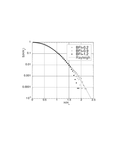
Figure 6: Survival function at x/L=2.8 for BFI0.2, crosses; BFI0.9, empty circles; BFI1.2 full circles.

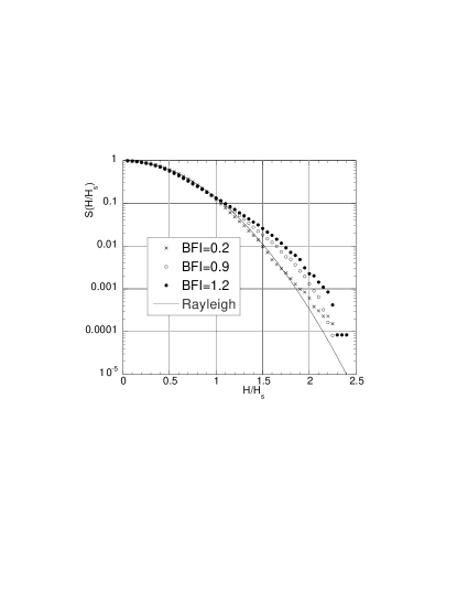
Figure 7: Survival function at x/L=18.5 for BFI0.2, crosses; BFI0.9, empty circles; BFI1.2 full circles.

Figure 8: Survival function at x/L=32.7 for BFI0.2, crosses; BFI0.9, empty circles; BFI1.2 full circles.

We then consider the probe at $x/L=18.5$, see Figure 7. While the data from BFI=0.2 are well described by the Rayleigh distribution, it is quite clear from the plot that the experimental data for BFI=0.9 and BFI=1.2 are substantially underestimated by the Rayleigh distribution. The curve for BFI=1.2 lies always on top of the one with BFI=0.9 and separates from the Rayleigh distribution at around $H/H_{s}$=1, which corresponds to a probability of 1/10 waves. A similar behavior is seen in Figure 8 at $x/L=32.7$.

We now compare in figure 9 our experimental results with Figure 6b in Onorato et al. (2000) that has been obtained by numerical simulations of the Dysthe equation, using as initial condition a JONSWAP spectrum with $\alpha=0.0081$ and $\gamma=6$. The Benjamin-Feir Index calculated for this spectrum has approximately the value BFI=0.9, therefore the probability distribution from numerical simulations is compared with our experimental data with the same BFI. The agreement is quite good.

Figure 9: Comparison of experimental results with results from numerical simulation of the Dysthe equation, see Onorato et al. (2000) for details of the numerical simulations.

V Discussion and conclusions

Recently a large number of papers that suggest that the modulational instability is a possible mechanism for explaining the formation of freak waves have appeared. A pioneering work in this context was performed by Trulsen and Dysthe (1997), who for the first time, considered seriously the possibility of describing nonlinear extreme waves using envelope equations. This work was also supported by a number of numerical and theoretical papers in which particular analytical solutions (“breathers” or more generally “unstable mode” solutions) of the NLS equations were considered as candidates for rogue waves (Peregrine (1983), Dysthe and Trulsen (1999), Osborne et al. (2000)). An important result that has been obtained from numerical simulations is that these “breather” solutions are very robust and can be excited also from random spectra (Onorato et al. (2003)). Their dynamics are quite different from the rest of the random wave field, they survive after interactions with other waves and periodically appear as large amplitude waves, while disappearing after some wavelengths. If the random wave field is very nonlinear (large steepness and small spectral width, corresponding to large BFI), the density of these objects increases, each of them having its own unique dynamics. Starting from an initial random wave field, they need several wavelengths (in our case it was about 25-30 wavelengths) to show up for the first time and, once they are formed, they continuously appear and disappear, nonlinearly interacting with the background wave field and each other. In a nonlinear wave field their presence is statistically significant, clearly leaving their signature in the survival function of wave heights. This phenomenological description, that has been conceived by us during many years of research with the envelope equations (see Onorato et al. (2000), Onorato et al. (2001), Onorato et al. (2002), Osborne et al. (2000)), is very consistent with the behaviour of real water waves. While for the NLS equation those objects survive forever in an ideal simulation (indeed it can be shown that they correspond to proper modes, called unstable modes, of the NLS equation and therefore correspond to constants of the motion, as for example solitons can be considered as constant of motion for the Korteweg de Vries equation), in real conditions higher-order effects can also take place: wave breaking and transverse instability can influence their dynamics and transform an unstable mode to another less nonlinear unstable mode. The experiments performed at Marintek support this picture. Indeed we have shown that the number of rogue waves (which in the language of the NLS equation roughly corresponds to the number of unstable modes) depend on the Benjamin- Feir Index of the initial spectrum. The presence of these modes determines the shape of the probability density function of wave heights. For nonlinearities consistent with water waves, the density of these modes is not very large, $3$x$10^{-3}$, therefore a large number of waves should be recorded in order to have reliable statistics. Even if we have collected a large number of data, sufficient to observe a clear departure from the Rayleigh distribution, we believe that statistics computed on even larger data sets should be used in order to model the tail of the survival function. The theory developed by Janssen (2003) should be closely compared with our experimental results (this is already part of an ongoing research program).

One of the limitations of our work that restrict us from extending our results in a straightforward manner to real wind waves is that our experiment has been performed in the case of infinite crested waves. For two dimensional propagation, numerical results and experimental work on the probability density function of wave heights are based on many fewer statistics, because numerics becomes much more expensive and experimental work requires large basins with wave makers capable of generating waves in different directions. Only a few results are available: Onorato et al. (2002), using the Dysthe equation in 2+1 dimensions with the exact linear dispersion relation, have shown that, if directional spreading is sufficiently narrow, the kurtosis of the surface elevation reaches values larger than 3 (the value for Gaussian distribution). This result is consistent with experimental work carried out in the Ocean Basin at Marintek, Stansberg (1994). It should be stated that in 2+1 dimensions, if the system is not continuously forced, four wave resonant interactions tend to broaden the spectrum and generate a tail of the form of $\omega^{-4}$ (Dysthe et al. (2003)); therefore the instability may take place only at the initial stages of a freely decaying simulation. Definitely more results including forcing and dissipation in 2+1 dimensions are needed for determining the role of the modulational instability for wind waves.

Acknowledgments

We thank P. Janssen and K. Trulsen for valuable discussions. Froydis Solaas is also acknowledged for technical support during the experiment. This research has been supported by the Improving Human Potential - Transnational Access to Research Infrastructures Programme of the European Commission under the contract HPRI-CT-2001-00176.

References

- Alber (2000) Alber, I. E. 1978 The effects of randomness on the stability of two dimensional surface wave trains. Proc. of Royal Soc. London A 636 525- 546
- Brandini (2001) Brandini, C. 2001 Nonlinear interaction processes in extreme wave dynamics Tesi di Dottorato, Università di Padova.
- Dommermuth and Yue (1987) Dommermuth, D.G. and Yue, D.K.P. 1987 A high-order spectral method for the study of nonlinear gravity waves J. Fluid Mech. 184 267 – 288.
- Dysthe and Trulsen (1999) Dysthe, K.B. and Trulsen, K. 1999 Note on breather type solutions of the NLS as a model for freak waves Physica Scripta T82 48–52.
- Dysthe et al. (2003) Dysthe, K.B., Trulsen, K., Krogstad, H.E. and Socquet-Juglard, H. 2003 Evolution of a narrow-band spectrum of random surface gravity waves J. Fluid Mech. 478 1–10.
- Earle, (1975) Earle, M. D. 1975 Extreme wave conditions during Hurricane Camille J. Geophyis. Res. 80 377–379.
- Forristall (1978) Forristall, G. Z. 1978 On the statistical distribution of wave heights in a storm. J. Geophys. Res. 83 2553–2558.
- Forristall (2000) Forristall, G. Z. 2000 Wave crest distributions: Observations and second-order theory J. Phys. Ocean. 30 1931–1943.
- Henderson et al. (1999) Henderson, K. L., Peregrine, D. H., Dold, J. W. 1999 Unsteady water wave modulations: fully nonlinear solutions and comparison with the nonlinear Schroedinger equation Wave Motion 29 341–361.
- Janssen (1991) Janssen, P. A. E. M. 1991 On nonlinear wave groups and consequences for spectral evolution. Directional Ocean Wave Spectra, R. C. Beal, Ed., The Johns Hopkins University Press, 46 -52.
- Janssen (2003) Janssen, P. A. E. M. 2003 Nonlinear Four-Wave Interactions and Freak Waves J. Phisical Ocean. 33, 863–883.
- Komen et al. (1994) Komen, G. J., Cavaleri, L., Donelan, M., Hasselmann, K., Hasselmann, H., Janssen, P. A. E. M 1994 Dynamics and modeling of ocean waves, Cambridge University Press
- Lavrenov (1998) Lavrenov, I. V. 1998 The wave energy concentration at the Agulhas current of South Africa Natural Hazards 17 117–127.
- Longuet-Higgins (1952) Longuet-Higgins, M. S. 1952 On the statistical distribution of the heights of sea waves. J. Marine Res. 11 1245–266.
- Longuet-Higgins (1980) Longuet-Higgins, M. S. 1980 On the distribution of the Heights of sea waves: Some effects of nonlinearity and finite band width J. Geophyis. Res. 85 1519–1523.
- Mori and Yasuda (2000) Mori, N. and Yasuda, T. 2000 Effects of higher-order nonlinear wave-wave interactions on deep-water waves. Rogue Wave 2000, (Ifremer, Brest 29-30 November 2000), eds. M. Olagnon and G.A. Athanassoulis 229–244.
- Mei (1983) Mei, C. C. 2000 he Applied Dynamics of Ocean Surface Waves (John Wiley, New York).
- Naess (1985) Naess, A. 1985 On the statistical distribution of crest to trough wave heights. Ocean Engineering 12 221-234.
- Onorato et al. (2000) Onorato, M., Osborne, A.R., Serio, M., Damiani, T. 2000 Occurrence of Freak Waves from Envelope Equations in Random Ocean Wave Simulations Rogue Wave 2000, (Ifremer, Brest 29,30 November 2000), eds. M. Olagnon and G.A. Athanassoulis 181-192.
- Onorato et al. (2001) Onorato, M., Osborne, A.R., Serio, Bertone, S. 2001 Freak waves in random oceanic sea states Phys. Rev. Letters 86, 5831–5834
- Onorato et al. (2002) Onorato, M., Osborne, A.R., Serio 2002 Extreme wave events in directional, random oceanic sea states Phys. of Fluids 14, L25–L28
- Onorato et al. (2003) Onorato, M., Osborne, A.R., Fedele, R., Serio, M. 2003 Landau damping and coherent structures in narrow-banded 1+1 deep water gravity waves Phys. Rev. E 67, 046305.
- Osborne et al. (2000) Osborne, A.R., Onorato, M., Serio, M. 2000 The nonlinear dynamics of rogue waves and holes in deep-water gravity wave trains Phys. Lett. A 275, 386–393.
- Peregrine (1983) Peregrine, D. H. 1983 Water waves, nonlinear Schroedinger equations and their solutions J. Austral. Math. Soc. B 25, 16–43.
- Rice (1944) Rice, S. O. 1944 Mathematical analysis of random noise Noise and Stochastic Processes (N. Wax, Ed.). New York: Dover Publications , Inc., 1954 133–294.
- Stansberg (1992) Stansberg, C. T. 1992 On spectral instabilities and development of nonlinearities in propagating deep-water wave trains Coastal Engineering, Procedings of the XXIII International Conference, Venice, ITALY, October 4-9, 658–671.
- Stansberg (1993) Stansberg, C. T. 1993 Propagation-dependent spatial variations observed in wave trains generated in a long wave tank. Data Report 490030.01 Marintek, Sintef group, Trondheim.
- Stansberg (1994) Stansberg, C. T. 1994 Effects from directionality and spectral bandwidth on nonlinear spatial modulations of deep water surface gravity wave trains. Coastal Engineering, Procedings of the XXIV International Conference, Kobe, Japan, October 23-28, 579–593.
- Stansberg (2000) Stansberg, C. T. 2000 Nonlinear Extreme Wave Evolution in Random Wave Groups International Society of Offshore and Polar Engineers, Seattle, USA, May 28-June 2, 2000 1-8.
- Trulsen and Dysthe (1997) Trulsen, K. and Dysthe, K.B. 1997 Freak Waves - A three-dimensional wave simulation Proceedings of the 21st Symposium on Naval Hydrodynamics (National Academy Press, Washington, DC, 1997), 550- 560
- Trulsen et al. (1999) Trulsen, K., Stansberg, C. T. and Velarde M.G. 1999 Laboratory Evidence of three dimensional frequency downshift of waves in a long tank Phys. of Fluids, 11, 235–237
- Tulin and Waseda (1999) Tulin, M. P. and Waseda, T. 1999 Laboratory observations of wave group evolution, including breaking effects textitJ. Fluid Mech. 378, 197– 232
- White and Fornberg (1998) White, B. S., Fornberg, B. 1998 On the chance of freak waves at the sea J. Fluid Mech. 255, 113–138