Faster than Lyapunov decays of classical Loschmidt echo

Abstract

We show that in the classical interaction picture the echo-dynamics, namely the composition of perturbed forward and unperturbed backward hamiltonian evolution, can be treated as a time-dependent hamiltonian system. For strongly chaotic (Anosov) systems we derive a cascade of exponential decays for the classical Loschmidt echo, starting with the leading Lyapunov exponent, followed by a sum of two largest exponents, etc. In the loxodromic case a decay starts with the rate given as twice the largest Lyapunov exponent. For a class of perturbations of symplectic maps the echo-dynamics exhibits a drift resulting in a super-exponential decay of the Loschmidt echo.

Analyzing the parametric stability of quantum dynamics through the so-called fidelity or Quantum Loschmidt Echo (QLE) has become increasingly popular and useful tool, either in the context of experiments with many-body systems Usaj , quantum computation Qcomp , or simple dynamical systems Peres ; Jalabert ; Prosen ; PZ ; Tomsovic ; Beenakker . The corresponding Classical Loschmidt Echo (CLE) has been defined PZ ; BC1 ; Eckhardt ; Veble , as

$$F(t)=\int{\rm d}^{N}{\bm{x}}\rho({\bm{x}})\rho_{\rm E}({\bm{x}},t)$$ (1)

where $\rho({\bm{x}})$ is an $L^{2}$ normalized non-negative initial density in $N=2d$-dimensional classical phase space with coordinates ${\bm{x}}$, and $\rho_{\rm E}({\bm{x}},t)$ is its image after the echo-dynamics, i.e. a composition of a hamiltonian flow with a slightly perturbed time-reversed hamiltonian flow. It has been found that for classically chaotic systems CLE follows QLE only for a short time that scales as $\log\hbar$. For longer times, CLE of chaotic systems has been shown to follow time correlation functions Veble . However, CLE is in itself an interesting quantity in classical statistical mechanics as it provides a way to quantify the old Loschmidt-Boltzmann controversy.

For shorter times, before the relaxation of the initially localized density under echo-dynamics takes place, it has been found numericallyBC1 that CLE decays exponentially with the rate given by the Lyapunov exponent. No classical mechanism for this phenomenon has been given, apart from the necessary correspondence with QLE for which a semiclassical theory of Lyapunov decay exists Jalabert . In this letter we report several surprising analytical results for the case of localized initial densities and for sufficiently weak perturbations: (i) In many-dimensional systems, a cascade of Lyapunov decays is predicted, with the exponents which are given as consecutive sums of largest few Lyapunov exponents. Hence precise conditions for previously observed simple Lyapunov decay are understood. (ii) In loxodromic case of degenerate largest Lyapunov exponent $\lambda_{1}=\lambda_{2}$ we find initial decay of CLE with exponent $2\lambda_{1}$. (iii) For maps under special conditions we find non-zero average drift of the echo-dynamics resulting in faster than exponential decay of CLE. The same results should apply for quantum fidelity (QLE) up to the log-time, namely until the Wigner function follows the classical density.

The propagation of classical densities in phase space is governed by the unitary Liouville evolution ${\hat{U}_{\delta}(t)}$

$$\frac{{\rm d}}{{\rm d}t}{\hat{U}}_{\delta}(t)={\cal{\hat{L}}}_{H_{\delta}({\bm{x}},t)}{\hat{U}}_{\delta}(t)$$ (2)

where ${\cal{\hat{L}}}_{\!A({\bm{x}},t)}=\left({\bm{\nabla}}\!A({\bm{x}},t)\right)\cdot{\rm\mathbf{J}}{\bm{\nabla}},$ $A$ is any observable, and

$$H_{\delta}({\bm{x}},t)=H_{0}({\bm{x}},t)+\delta V({\bm{x}},t),$$ (3)

is a generally time-dependent family of Hamiltonians with perturbation parameter $\delta$. Matrix ${\rm\mathbf{J}}$ is the usual symplectic unit. Similarly, ${\rm d}{\hat{U}}^{\dagger}_{\delta}(t)/{\rm d}t=-{\hat{U}}^{\dagger}_{\delta}(t){\cal{\hat{L}}}_{H_{\delta}({\bm{x}},t)}.$ The classical echo propagator that composes perturbed forward evolution with the unperturbed backward evolution is also unitary and is given by

$${\hat{U}}_{\rm E}(t)={\hat{U}}^{\dagger}_{0}(t)\,{\hat{U}}_{\delta}(t).$$ (4)

Using eqs. (2,3,4) and writing ${\hat{U}}_{\delta}(t)={\hat{U}}_{0}(t){\hat{U}}_{\rm E}(t)$ we get

$$\frac{{\rm d}}{{\rm d}t}{\hat{U}}_{\rm E}(t)=\left\{{\hat{U}}_{0}^{\dagger}(t){\cal{\hat{L}}}_{\delta V({\bm{x}},t)}{\hat{U}}_{0}(t)\right\}{\hat{U}}_{\rm E}(t).$$ (5)

The classical dynamics has the nice property that the evolution is governed by characteristics that are simply the classical phase space trajectories, so the action of the evolution operator on any phase space density is given as ${\hat{U}}_{0}(t)~{}\rho=\rho\circ{\bm{\phi}}_{t}^{-1},$ where $\phi_{t}^{-1}$ denotes the backward (unperturbed) phase space flow from time $t$ to $0$. Similarly, ${\hat{U}}_{0}^{\dagger}(t)~{}\rho=\rho\circ{\bm{\phi}}_{t},$ where $\phi_{t}$ represents the forward phase space flow from time $0$ to time $t$. Here and in the following we assume the dynamics to start at time $0$.

We note that echo-dynamics (4) can be treated as Liouvillian dynamics in interaction picture, since

$$\left\{{\hat{U}}_{0}^{\dagger}(t){\cal{\hat{L}}}_{A({\bm{x}},t)}{\hat{U}}_{0}(t)\rho\right\}({\bm{x}})=$$ (6)

$$={\hat{U}}_{0}^{\dagger}(t)\left({\bm{\nabla}}_{{\bm{x}}}A({\bm{x}},t)\right)\cdot{\rm\mathbf{J}}{\bm{\nabla}}_{{\bm{x}}}\rho\left({\bm{\phi}}_{t}^{-1}({\bm{x}})\right)=$$

$$=\left({\bm{\nabla}}_{{\bm{\phi}}_{t}({\bm{x}})}A({\bm{\phi}}_{t}({\bm{x}}),t)\right)\cdot{\rm\mathbf{J}}{\bm{\nabla}}_{{\bm{\phi}}_{t}({\bm{x}})}\rho\left({\bm{\phi}}_{t}^{-1}\left({\bm{\phi}}_{t}({\bm{x}})\right)\right)=$$

$$=\left({\bm{\nabla}}_{{\bm{x}}}A({\bm{\phi}}_{t}({\bm{x}}),t)\right)\cdot{\rm\mathbf{J}}{\bm{\nabla}}_{{\bm{x}}}\rho({\bm{x}})=\left\{{\cal{\hat{L}}}_{A\left({\bm{\phi}}_{t}({\bm{x}}),t\right)}~{}\rho\right\}({{\bm{x}}}).$$

In the last line we used the invariance of the Poisson bracket under the flow. This extends eq. (5) to form (2)

$$\frac{{\rm d}}{{\rm d}t}{\hat{U}}_{\rm E}(t)={\cal{\hat{L}}}_{H_{\rm E}({\bm{x}},t)}~{}{\hat{U}}_{\rm E}(t)$$ (7)

where the echo Hamiltonian is given by

$$H_{\rm E}({{\bm{x}}},t)=\delta V\left({\bm{\phi}}_{t}({\bm{x}}),t\right).$$ (8)

The function $H_{\rm E}$ is nothing but the perturbation part $\delta V$ of the original Hamiltonian, which, however, is evaluated at the point that is obtained by forward propagation with the unperturbed original Hamiltonian. It is important to stress that this is not a perturbative result but an exact expression. Also, even if the original Hamiltionian system was time independent, the echo dynamics obtains an explicitly time dependent form. Trajectories of the echo-flow are given by Hamilton equations

$$\dot{{\bm{x}}}={\rm\mathbf{J}}~{}{\bm{\nabla}}H_{\rm E}({\bm{x}},t).$$ (9)

At this point we limit our discussion only to time independent original Hamiltonians and perturbations. Slightly more general case of periodically driven systems reducible to symplectic maps shall also be discussed later.

Inserting (8) into eq. (9) yields

$$\dot{{\bm{x}}}=\delta{\rm\mathbf{J}}{\bm{\nabla}}_{{\bm{x}}}V({\bm{\phi}}_{t}({\bm{x}}))=\delta{\rm\mathbf{J}}{{\rm\mathbf{M}}_{t}^{T}({\bm{x}})}({\bm{\nabla}}V)({\bm{\phi}}_{t}({\bm{x}})).$$ (10)

Here we have introduced the stability matrix ${\rm\mathbf{M}}_{t}({\bm{x}})$, $[{\rm\mathbf{M}}_{t}({\bm{x}})]_{i,j}=\partial_{j}[{\bm{\phi}}_{t}({\bm{x}})]_{i}$. From now on we assume that the flow ${\bm{\phi}}_{t}$ is Anosov. To understand the dynamics (10) we need to explore the properties of ${\rm\mathbf{M}}_{t}$. We start by writing the matrix ${\rm\mathbf{M}}_{t}^{T}({\bm{x}}){\rm\mathbf{M}}_{t}({\bm{x}})=\sum_{j}e^{2\lambda_{j}t}d_{j}^{2}({\bm{x}},t){\bm{v}}_{j}({\bm{x}},t)\otimes{\bm{v}}_{j}({\bm{x}},t)$ expressed in terms of orthonormal eigenvectors ${\bm{v}}_{j}({\bm{x}},t)$ and eigenvalues $d_{j}^{2}({\bm{x}},t)\exp(2\lambda_{j}t)$. After the ergodic time $t_{\rm e}$ necessary for the echo trajectory to explore the available region of phase space, Osledec theoremOsledec guarantees that the eigenvectors of this matrix converge to Lyapunov eigenvectors being independent of time, while $d_{j}({\bm{x}},t)$ grow slower than exponentially, so the leading exponential growth defines the Lyapunov exponents $\lambda_{j}$. Similarly, the matrix ${\rm\mathbf{M}}_{t}({\bm{x}}){\rm\mathbf{M}}_{t}^{T}({\bm{x}})=\sum_{j}e^{2\lambda_{j}t}c_{j}^{2}({\bm{x}}_{t},t){\bm{u}}_{j}({\bm{x}}_{t},t)\otimes{\bm{u}}_{j}({\bm{x}}_{t},t),$ where ${\bm{x}}_{t}={\bm{\phi}}_{t}({\bm{x}})$, has the same eigenvalues [$c^{2}_{j}({\bm{x}}_{t},t)\equiv d^{2}_{j}({\bm{x}},t)$], and its eigenvectors depend on the final point ${\bm{x}}_{t}$ only, as the matrix in question can be related to the backward evolution. The vectors $\{{\bm{u}}_{j}({\bm{x}}_{t})\}$, $\{{\bm{v}}_{j}({\bm{x}})\}$, constitute left, right, part, respectively, of the singular value decomposition of ${\rm\mathbf{M}}_{t}({\bm{x}})$, so we write for $t\gg t_{\rm e}$

$${\rm\mathbf{M}}_{t}({\bm{x}})=\sum_{j=1}^{N}\exp(\lambda_{j}t)~{}{\bm{e}}_{j}({\bm{\phi}}_{t}({\bm{x}}))\otimes{\bm{f}}_{j}({\bm{x}})$$ (11)

assuming that the limits ${\bm{e}}_{j}({\bm{x}})=\lim_{t\to\infty}c_{j}({\bm{x}},t){\bm{u}}_{j}({\bm{x}},t)$, ${\bm{f}}_{j}({\bm{x}})=\lim_{t\to\infty}d_{j}({\bm{x}},t){\bm{v}}_{j}({\bm{x}},t)$ exist. Rewriting eq. (10) by means of eq. (11) we obtain

$$\dot{{\bm{x}}}=\delta\sum_{j=1}^{N}\exp(\lambda_{j}t)~{}W_{j}({\bm{\phi}}_{t}({\bm{x}}))~{}{\bm{h}}_{j}({\bm{x}})$$ (12)

where ${\bm{h}}_{j}({\bm{x}})={\rm\mathbf{J}}{\bm{f}}_{j}({\bm{x}})$, and introducing new observables

$$W_{j}({\bm{x}})={\bm{e}}_{j}({\bm{x}})\cdot{\bm{\nabla}}V({\bm{x}}).$$ (13)

At this point it is perhaps necessary to discuss the nature of the vector fields ${\bm{e}}_{j}({\bm{x}})$, ${\bm{f}}_{j}({\bm{x}})$ remark . While the theorem Osledec guarantees the existence of these directions, the actual sizes of these fields as given by $c_{j}$, $d_{j}$ are not yet well understood. Numerical data suggest that these quantities do converge as $t\to\infty$ for an Anosov system.

For small perturbations the echo trajectories remain close to initial point ${\bm{x}}(0)$ for times large in comparison to the internal dynamics of the system ($t_{\rm e}$, Lyapunov times, decay of correlations, etc), and in this regime the echo evolution can be linearly decomposed along different independent directions ${\bm{h}}_{j}({\bm{x}}(0))$

$${\bm{x}}(t)={\bm{x}}(0)+\sum_{j=1}^{N}y_{j}(t)~{}{\bm{h}}_{j}({\bm{x}}(0)).$$ (14)

For longer times, the point ${\bm{x}}(t)$ moves away from the initial point, but the dynamics is still governed by the local unstable vectors at the evolved point. Therefore the decay of fidelity is governed by the spreading of the densities along the conjugated unstable manifolds defined by the vector field ${\bm{h}}({\bm{x}})$.

Inserting (14) into (12) we obtain for each direction ${\bm{h}}_{j}$

$$\dot{y}_{j}=\delta~{}\exp(\lambda_{j}t)W_{j}({\bm{\phi}}_{t}({\bm{x}})).$$ (15)

For stable directions with $\lambda_{j}<0$, clearly after a certain time the variable $y_{j}$ becomes a constant of the order $\delta$.

For unstable directions with $\lambda_{j}>0$, we introduce $z_{j}$ as $y_{j}=\delta\exp(\lambda_{j}t)z_{j}$ and rewrite the above equation as

$$\dot{z}_{j}+\lambda_{j}z_{j}=W_{j}({\bm{\phi}}_{t}({\bm{x}})).$$ (16)

The right hand side of this equation is simply the evolution of the observable $W_{j}$ starting from a point in phase space ${\bm{x}}={\bm{x}}(0)$. Due to assumed ergodicity of the flow ${\bm{\phi}}_{t}$, $W_{j}({\bm{\phi}}_{t}({\bm{x}}))$ has well defined and stationary statistical properties such as averages and correlation functions. Thus the solution $z_{j}(t)$ of the linear damped equation (16) has also stationary statistics and well defined time- and $\delta$-independent probability distribution $P_{j}(z_{j})$. Its moments can be expressed in terms of moments and correlation functions of $W_{j}$, in particular $\overline{W_{j}}=0$ firstmoment . The analysis remains valid in a general case of explicitly time-dependent $W_{j}$ remark .

Going back to the original coordinate $y_{j}$ we obtain its distribution as $K_{j}(y_{j})=P_{j}(z_{j}){\rm d}z_{j}/{\rm d}y_{j}$, or $K_{j}(y_{j})=P_{j}\left(\exp(-\lambda_{j}t)y_{j}/\delta\right)\exp(-\lambda_{j}t)/\delta.$ This probability distribution tells us how, on average, points within some initial (small) phase space set of characteristic diameter $\nu$ spread along locally well defined unstable Lyapunov direction $j$ and therefore represents an averaged kernel of the evolution of such densities along this direction. Starting from the initial localized density $\rho_{0}$, of small width $\nu$ such that the decomposition (14) does not change appreciably along $\rho_{0}$, the echo dynamics for densities solves as $\rho_{t}({\bm{y}})=\int{\rm d}^{N}{\bm{y}}^{\prime}\rho_{0}({\bm{y}}^{\prime})\prod_{j}K_{j}(y_{j}-y_{j}^{\prime}).$ For stable directions $j$ we set $K_{j}(y_{j})=\delta(y_{j})$, as the shift of $y_{j}$ (of order $\delta$) can be neglected as compared to unstable directions. This also implies that the assumption $\delta\ll\nu$ is necessary in order to get any echo at all after not too short times. CLE (1) can now be written as $F(t)=\int{\rm d}^{N}{\bm{y}}~{}\rho_{0}({\bm{y}})~{}\rho_{t}({\bm{y}})$. As long as the width $\nu_{j}$ of $\rho_{0}$ along the unstable direction $j$ is much larger than the width of the kernel $K_{j}$, there is no appreciable contribution to the fidelity decay in that direction. At time

$$t_{j}=(1/\lambda_{j})\log(\nu_{j}/(\delta\gamma_{j})),$$ (17)

where $\gamma_{j}$ is a typical width of the distribution $P_{j}$, the width of the kernel is of the order of the width of the distribution along the chosen direction. After that time, the overlap between the two distributions along the chosen direction starts to decay with the same rate as the value of the kernel in the neighborhood of $y_{j}=0$, which is $\propto\exp(-\lambda_{j}t)$. The total overlap decays as

$$F(t)\approx\prod_{j;~{}t_{j}<t}\exp\left[-\lambda_{j}(t-t_{j})\right],$$ (18)

where only those unstable directions contribute to the decay for which $t_{j}>t$. As the time $t_{j}$ is shorter the higher the corresponding Lyapunov exponent $\lambda_{j}$, fidelity will initially decay with the largest Lyapunov exponent $\lambda_{1}$. In chaotic systems with more than two degrees of freedom we, however, expect to observe an increase of decay rate after the time $t_{2}$, etc. Eq. (18) provides good description for CLE as long as $F(t)$ does not approach the saturation value $F_{\infty}\sim\nu^{N}$ where the asymptotic decay of CLE is then given by leading Perron-Frobenius eigenvalue Veble .

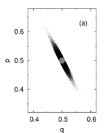
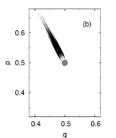
Figure 1: Density evolution of echo-dynamics for the perturbed cat map [eq. (19), $\mu=0.3$]. The initial density is a characteristic function on the circle (gray) centered at $(q,p)=(0.5,0.5)$ having the radius $0.01$, while the evolved density at the time $t=21$ is represented by $10^{5}$ dots. Figures (a,b) refer to corresponding cases for perturbations without and with drift, respectively ($\delta=10^{-9}$, see text for details).

Figure 2: CLE as a function of time for the same conditions as in fig. 1 except using $10^{6}$ points. The circles refer to the case (a) (no drift), chain line is the theoretical Lyapunov decay with $\lambda_{1}=0.958$, and the triangles refer to the ballistic case (b) (drift). In both cases the fidelity saturates at the plateau (dotted line) given by the relative volume (area) of the initial set.

Figure 3: CLE for two examples of 4D cat maps perturbed as explained in text. Triangles refer to doubly-hyperbolic case where initial set was a 4-cube $[0.1,0.11]^{4}$, and $\delta=2\cdot 10^{-4}$, whereas circles refer to loxodromic case where initial set was $[0.1,0.15]^{4}$, and $\delta=3\cdot 10^{-3}$. In both cases initial density was sampled by $10^{9}$ points. Chain lines give exponential decays with theoretical rates, $\lambda_{1}=1.65,\lambda_{1}+\lambda_{2}=2.40$ (doubly-hyperbolic), and $2\lambda_{1}=1.06$ (loxodromic).

Though the above theory has been developed for smooth flows, the generalization to ergodic symplectic maps on bounded phase space ${\cal M}$ is straightforward. We adopt notation of Ref. PZ , sect. 4: ${\bm{\phi}}\equiv{\bm{\phi}}_{1}$, discrete time $t$ is an integer and a general small perturbation is given by a composition ${\bm{\phi}}_{\delta}={\bm{\phi}}\circ{\bm{g}}_{\delta}$ with a near-identity map ${\bm{g}}_{\delta}$ generated by a vector field ${\bm{a}}({\bm{x}})$, ${\rm d}{\bm{g}}_{\delta}/{\rm d}\delta={\bm{a}}({\bm{g}}_{\delta})$ with initial condition ${\bm{g}}_{0}({\bm{x}})={\bm{x}}$. For the perturbed map to remain symplectic we write ${\bm{a}}({\bm{x}})={\rm\mathbf{J}}{\bm{\nabla}}V({\bm{x}})$ for some potential $V({\bm{x}})$. We note that on compact phase space $V({\bm{x}})$ does not need to be unique and continuous, e.g. for a unit 2-torus $V(q+1,p)=V(q,p)+\alpha,V(q,p+1)=V(q,p)+\beta$ where $\alpha,\beta$ are arbitrary constants. Provided hyperbolic orbits with inversion do not exist, $\eta\equiv 0$ remark , one finds a non-vanishing drift of echo-dynamcis, $\overline{W}_{j}\neq 0$, resulting in a possible super-exponential decay of CLE if the mean $\overline{W_{j}}/\lambda_{j}$ of the distribution $P_{j}(z_{j})$ is larger than its width $\gamma_{j}$.

In order to illustrate super-exponential versus exponential decay of CLE we consider the perturbed cat map

$$\overline{p} = p+q-\frac{\mu}{2\pi}\sin(2\pi q)+\delta s(q),\quad\mu\in[0,1)$$

$$\overline{q} = q+\overline{p}.$$ (19)

The perturbation was chosen either as: (a) $s(q)=\sin(2\pi q)/(2\pi)$, or (b) $s(q)=1/(2\pi)$ where the perturbation is a shift in phase space. The main difference between the two is that the case (a) corresponds to zero drift since a unique smooth potential exists ($\alpha=\beta=0$), while in case (b) ${\bm{a}}={\rm const}\neq 0$ and the Lyapunov fields have a predominant direction in phase space for this system, e.g. for the unperturbed cat map ($\mu=0$) ${\bm{e}}({\bm{x}}),{\bm{f}}({\bm{x}}),{\bm{h}}({\bm{x}})$ are constant. Since the perturbed cat has no orbits with inversionremark the corresponding phase space observable $W_{j}$ for the case (b) has a distinct nonzero average value, causing the kernel $K_{j}$ to drift exponentially in time. The difference in the qualitative nature of the two decays is shown in figure 1. In figure 2 we show the behaviour of fidelity as a function of time for the two cases, where a super-exponential decay is observed in the case of drift.

Another result, which applies only to systems with two or more unstable directions, is the occurrence of decays which are exponential but faster than Lyapunov. In the case of well separated individual Lyapunov exponents the decay is expected to go through a cascade of increasing decay rates given by (18), whereas in the loxodromic case $\lambda_{1}=\lambda_{2}$ the rate is $2\lambda_{1}$. We illustrate this numerically for 4D cat maps Rivas : ${\bm{x}}^{\prime}={\rm\mathbf{C}}{\bm{x}}\pmod{1},$ ${\bm{x}}\in[0,1)^{4}$, and

$${\rm\mathbf{C}}_{\rm d-h}=\left[\begin{array}[]{rrrr}2&-2&-1&0\\ -2&3&1&0\\ -1&2&2&1\\ 2&-2&0&1\end{array}\right],\ {\rm\mathbf{C}}_{\rm lox}=\left[\begin{array}[]{rrrr}0&1&0&0\\ 0&1&1&0\\ 1&-1&1&1\\ -1&-1&-2&0\end{array}\right]$$

are two examples representing the doubly-hyperbolic and loxodromic case. Matrix ${\rm\mathbf{C}}_{\rm d-h}$ has the unstable eigenvalues $\approx 5.22,2.11$, while the large eigenvalues of ${\rm\mathbf{C}}_{\rm lox}$ are $\approx 1.70\exp(\pm{\rm i}1.12)$. The perturbation for both cases was done by performing an additional mapping at each timestep $\bar{x}_{1}=x^{\prime}_{1}+\delta\sin\left(2\pi x_{3}\right)\pmod{1}$, $\bar{x}_{2,3,4}=x^{\prime}_{2,3,4}$. In figure 3 we show the two types of decay which agree with theoretical predictions.

In conclusion, we have developed a theory for short-time decay of CLE based on classical interaction picture. Our theory predicts several new phenomena, in particular a cascade of exponential decays in systems with more than one unstable direction and doubly-Lyapunov decay for the particular case of loxodromic stability. Besides being related to quantum computation, our results for systems with many degrees of freedom provide a way to understand macroscopic irreversibility in classical statistical mechanics.

We acknowledge useful discussion with T.H.Seligman and financial support by the Ministry of Education, Science and Sport of Slovenia, and in part by the U.S. ARO grant DAAD19-02-1-0086.

References

(1) H. M. Pastawski et al. Physica A 283, 166 (2000).
(2) M. A. Nielsen and I. L. Chuang,
Quantum computation and quantum information (Cambridge UP, 2001).
(3) A. Peres, Phys. Rev. A 30, 1610 (1984).
(4)
R. A. Jalabert and H. M. Pastawski, Phys. Rev. Lett. 86, 2490 (2001).
(5) T. Prosen, Phys. Rev. E 65, 036208 (2002).
(6) T. Prosen and M. Žnidarič, J. Phys. A 35, 1455 (2002).
(7) N. R. Cerruti and S. Tomsovic, Phys. Rev. Lett. 88, 054103 (2002).
(8) Ph. Jacquod et al. Phys. Rev. E 64, 055203(R) (2001).
(9) G. Benenti and G. Casati, Phys. Rev. E 65, 066205 (2002).
(10) B. Eckhardt, J. Phys. A: Math. Gen 36, 371 (2003).
(11) G. Benenti, G. Casati and G. Veble, Phys. Rev. E 67, 055202 (2003).
(12) V. I. Osledec, Moscow. Math. Soc. 19, 197 (1968).
(13) We note that signs of the fields
are not unique provided the flow has
hyperbolic periodic orbits with inversion. In such a case, the explicitly
time-dependent observables
should be defined
with an additional sign-factor which counts the number of
inversions of the vector field along the trajectory,
(14) It is equivalent to show that ,
for finite but arbitrary long , which follows from integrating by parts the rightmost side of eq.
(10).
(15) A. M. F. Rivas et al, Nonlinearity 13, 341 (2000).