Rotating Spiral Waves with Phase-Randomized Core in Non-locally Coupled Oscillators

Abstract

Rotating spiral waves with a central core composed of phase-randomized oscillators can arise in reaction-diffusion systems if some of the chemical components involved are diffusion-free. This peculiar phenomenon is demonstrated for a paradigmatic three-component reaction-diffusion model. The origin of this anomalous spiral dynamics is the effective non-locality in coupling, whose effect is stronger for weaker coupling. There exists a critical coupling strength which is estimated from a simple argument. Detailed mathematical and numerical analyses are carried out in the extreme case of weak coupling for which the phase reduction method is applicable. Under the assumption that the mean field pattern keeps to rotate steadily as a result of a statistical cancellation of the incoherence, we derive a functional self-consistency equation to be satisfied by this space-time dependent quantity. Its solution and the resulting effective frequencies of the individual oscillators are found to agree excellently with the numerical simulation.

I INTRODUCTION

Rotating spiral waves represent a most universal form of patterns appearing in reaction-diffusion systems and other dissipative media of oscillatory and excitable nature. Most of the recent experimental and theoretical studies on rotating spiral waves in reaction-diffusion systems have focused on their complex behavior such as core meandering in 2DBarkley (1994, 1995), manipulation of the pattern using photo-sensitive BZ reactionKheowan et al. (2001); Mihaliuk et al. (2002), and the topology and dynamics of the singular filaments of 3D scroll wavesWinfree (1990); Keener and Tyson (1992); Alonso et al. (2003). Slightly deviated from this mainstream, the possibility of a new type of spiral dynamics caused by a universal mechanism was proposed recently by the present authorsKuramoto and Shima (2003). This is characterized by the appearance of a local group of oscillators near the center of spiral rotation where the oscillators behave individually rather than collectively. A simple class of three-component reaction-diffusion systems involving two diffusion-free components and an extra diffusive component proved to exhibit this type of anomaly. Here the last component plays the role of a coupling agent allowing the otherwise independent local oscillators to communicate with each other, where the communication takes place non-locally. The crucial parameter to this peculiar spiral dynamics is the strength of the non-local coupling. If it is sufficiently large, the characteristic wavelength of the pattern, especially the radius of the spiral core, becomes longer than the coupling radius. Consequently, the coupling becomes effectively local, i.e., diffusive, and there is nothing peculiar about the resulting spiral pattern. As the coupling becomes weaker, in contrast, its non-local nature becomes stronger, and finally a small group of phase-randomized oscillators starts to be created near the center of rotation. We find in the present paper that under certain conditions the phase-randomized core is stationary in a statistical sense. This allows us to formulate a statistical theory with which the entire system dynamics, collective and individual, can completely be specified. Actually, the exact self-consistent theory developed here provides a rare example of statistical theories associated with large systems of limit-cycle oscillators when spatial degrees of freedom are involved.

The organization of the present paper is the following. In Sec. II, we start with a brief review of some general features of the three-component reaction-diffusion model introduced earlier, and show how it is reduced to a two-component system of non-locally coupled oscillators. Then, adopting a specific model for the local oscillators, we present some results of our numerical simulation revealing the fact that the spiral core can be coherent or incoherent depending on the coupling parameter. We shall also see that the critical coupling strength associated with the onset of incoherence can be estimated from a simple argument. Section III and IV, each devoted to numerical and mathematical analyses, are concerned with the special situation where the coupling is sufficiently weak. Then the so-called phase reduction method is applicable, by which a phase oscillator model with non-local coupling is derived. What is remarkable is the fact that, as opposed to the conventional view, description of the spiral dynamics in terms of the phase oscillator model does not lead to a topological contradiction but can even provide its precise description. Using this non-local phase model, we develop a mean field theory similar to Kuramoto’s 1975 theory on the onset of collective synchronization in globally coupled oscillatorsKuramoto (1975). The present mean field theory is based on the assumption of steady rotation of the mean field pattern. Owing to this assumption, we can derive a functional self-consistency equation to be satisfied by the mean field. Numerical solution of this functional equation is confirmed to agree exceedingly well with the simulation results.

II REACTION-DIFFUSION MODEL AND ITS REDUCED FORM

II.1 Effective Non-locality in Reaction-Diffusion Systems

Consider a three-component reaction-diffusion system of the following form.

$$\partial_{t}X(\mbox{\boldmath$r$},t) =f(X,Y)+K(B-X),$$ (1)

$$\partial_{t}Y(\mbox{\boldmath$r$},t) =g(X,Y),$$ (2)

$$\tau\partial_{t}B(\mbox{\boldmath$r$},t) =-B+D\nabla^{2}B+X.$$ (3)

The system is supposed to extend sufficiently in two dimensions. The above model has recently been used as a paradigmatic model for the study of various aspects of self-oscillatory fields where the effective non-locality in coupling plays a crucial roleKuramoto and Shima (2003); Kuramoto et al. (2000); Tanaka and Kuramoto (2003). The first two equations with $K=0$ represent a local limit-cycle oscillator. Our system may therefore be interpreted as a continuum limit of a large assembly of oscillators without direct mutual coupling which are suspended in a diffusive chemical with concentration $B$. The last quantity plays the role of a coupling agent only by which the local oscillators can mutually communicate. For simplicity, a cross coupling between the local oscillators and the diffusive field has been introduced in a linear form and only between $X$ and $B$. The coupling term $K(B-X)$ may equivalently be replaced with a more natural form $KB$ if $f(X,Y)$ is suitably redefined, but we will work with the first form for its mathematical convenience to be seen later.

Our system, possibly with various modifications and generalizations, bears some resemblance to biological populations of oscillatory and excitable cells such as suspensions of yeast cells under glycolysis and slime mold amoebae in a certain phase of their life cycleTyson et al. (1989); Goldbeter (1996); Danø et al. (2002). One may also note some similarity of the above model to the recently developed version of the Belousov-Zhabotinsky reaction using water-in-oil AOT micro-emulsionVang and Epstein (2001); Vanag and Epstein (2002); Vang and Epstein (2003). Some of the interesting theoretical aspects of our reaction-diffusion model have already been reported Kuramoto and Shima (2003); Kuramoto et al. (2000); Tanaka and Kuramoto (2003).

When the characteristic time scale of $B$, denoted by $\tau$, is sufficiently small, this component can be eliminated adiabatically by solving the equation

$$0=-B+D\nabla^{2}B+X.$$ (4)

The solution of the above equation is expressed in terms of the Green function $G(\mbox{\boldmath$r$})$ in the form

$$B(\mbox{\boldmath$r$},t)=\int G(\mbox{\boldmath$r$}-\mbox{\boldmath$r$}^{\prime})X(\mbox{\boldmath$r$}^{\prime},t)d\mbox{\boldmath$r$}^{\prime}.$$ (5)

If our system is infinitely extended, $G(\mbox{\boldmath$r$})$ is radially symmetric, and for spatial dimension two it is given by a modified Bessel function of the second kind with the characteristic length scale $r_{0}=\sqrt{D}$, i.e.,

$$G(r)=\frac{1}{2\pi r_{0}^{2}}\;K_{0}\!\!\left(\frac{r}{r_{0}}\right),\quad r=|\mbox{\boldmath$r$}|.$$ (6)

Note that the above $G(r)$ satisfies the normalization condition $\int G(r)d\mbox{\boldmath$r$}=1$, and behaves asymptotically as $G(r)\sim\exp(-r/r_{0})/\sqrt{r/r_{0}}$ for $r\gg r_{0}$. We may call $B(\mbox{\boldmath$r$},t)$ the space-time dependent mean field because this quantity roughly represents a mean value of $X(\mbox{\boldmath$r$}^{\prime},t)$ over a circular domain with the radius of $O(\sqrt{D})$ centered at $r$. Our original reaction-diffusion system has now been reduced to the system of Eqs. (1), (2) and (5), which represents a two-component oscillatory field with non-local coupling.

Suppose that we change parameter $K$, which measures, in terms of the reduced system, the strength of the non-local coupling. If $K$ is sufficiently large, the characteristic wavelength of the pattern, denoted by $l_{p}$, will be far longer than the coupling radius (as is justified below). Then the long-wavelength approximation can applied to Eq. (5), giving $K(B-X)\simeq\tilde{D}\nabla^{2}X$, where $\tilde{D}=KD$. Thus, the non-local coupling practically reduces to a diffusive coupling in this strong-coupling case. One may check the consistency of the above argument by noticing the fact that the result of this diffusion-coupling approximation itself tells that $l_{p}$ estimated from Eq. (1) scales like $l_{p}\sim\sqrt{\tilde{D}}=\sqrt{KD}$. Thus, sufficiently large $K$ implies $l_{p}$ larger than the coupling radius $\sqrt{D}$, so that our long-wavelength assumption proves to be consistent. In any case, our system for strong coupling reduces to a two-component reaction-diffusion system, which, however, is of our little concern in the present paper.

The situation of our interest is the opposite case in which $K$ is so small that $l_{p}$ becomes comparable with or even smaller than the coupling radius of $O(\sqrt{D})$. Then the diffusion-coupling approximation breaks down, and the system comes to behave in an unusual manner. It should be noted here that the evolution equations themselves are free of characteristic length scale below the coupling radius. Therefore, once $l_{p}$ comes to fall within the coupling radius, or equivalently, once spatial variations with wavelengths smaller than the coupling radius are generated spontaneously, then there is no reason why spatial variations of even smaller wavelengths should not occur. We suspect therefore that the kind of anomaly of our concern might be characterized by a fragmentation of the pattern down to infinitesimal spatial scales. This is actually the case, which we show below by presenting some numerical results on the non-locally coupled system given by Eqs. (1), (2) and (5) with specific forms for $f$ and $g$.

II.2 Case of the FitzHugh-Nagumo Oscillators

As a simple model for the local oscillators, let us consider the FitzHugh-Nagumo model given by

$$f=\sigma^{-1}\{(X-X^{3})-Y\},\quad g=aX+b.$$ (7)

We fix the parameter values as $a=1.0$, $b=0.2$ and $\sigma=0.1$, so that the system is well in the self-oscillatory regime.

We carried out a numerical analysis on a non-locally coupled field of oscillators described by Eqs. (1), (2), (5) and (7). The system is defined over the square domain $x,y\in[0,L]$ where $B$ satisfies the free boundary conditions, namely, the vertical component of $\nabla B$ to the boundaries vanishes. Thus, the Green function $G$ differs in this case from the form given by Eq. (6) especially near the boundaries. In practical numerical simulation, our continuous space was replaced with a square lattice of oscillators of $N\times N$ lattice points, a typical value of $N$ being 2048. At each time step, $B$ was calculated from Eq. (5), or equivalently Eq. (4), by means of a spatial Fourier transform. The 4th order Runge-Kutta scheme was adopted for the time-integration of Eqs. (1) and (2).

Some numerical results for two representative values of $K$ are illustrated in FIG. 1. Figure 1 (a) to (c) correspond to the case of large $K$. They respectively show an overall spiral pattern, its blowup near the center of rotation, and the phase portrait of the pattern in the $X$-$Y$ plane. The last quantity is given by a set of $N^{2}$ points in the $X$-$Y$ plane each representing the state of a local oscillator at a given time. In usual reaction-diffusion systems such as those modeled with two-component reaction-diffusion equations, the phase portrait associated with a spiral pattern is considered to form a simply connected object involving a phase singularity. This is a natural consequence of the homeomorphism which is supposed to characterize the mapping between the physical space and the state space. The same property seems to hold in the present case of large $K$, and this is consistent with the fact already noted that for sufficiently strong coupling our system reduces to a two-component reaction-diffusion system.

Figure 1 (d) to (f) correspond to the case of small $K$. The overall spiral pattern does not seem qualitatively different from that for large $K$. As is clear from Fig. 1 (e), however, closer observation of the core structure reveals a completely new feature of the pattern. This is the appearance of a group of oscillators near the center of rotation where the oscillators seem to behave individually rather than collectively. The corresponding phase portrait, which is presented in FIG. 1 (f), no longer seems to tend to a simply connected object in the continuum limit. The hole created in the phase portrait gives a clear indication of the breakdown of the homeomorphism mentioned above. It may alternatively be said that a pair of local oscillators situated infinitely close to each other are not always so close in the state space, which says nothing but a loss of spatial continuity of the pattern. At the same time, the phase singularity, which is generally considered as a central characteristic shared by spiral patterns, seems to be lost, i.e., the pattern no longer seems to involve a special local oscillator for which the phase cannot be defined.

The origin of the spiral core anomaly of this kind may qualitatively be understood in the following way. Our primary question is why the core region is the most fragile part of the pattern with respect to the collapse of spatial continuity. In order to see why, it is convenient to look upon Eqs. (1) and (2) as describing a single oscillator driven by a forcing field $B$ whose spatial variation is expected to be relatively smooth from its definition given by Eq. (4). Wherever the oscillation amplitude of $B$ is sufficiently large, the oscillators will individually synchronize with the motion of $B$, so that a local group of such oscillators will mutually synchronize also. The corresponding local pattern will then look continuous and smooth. This is considered to be the case for those oscillators far apart from the central core, because the oscillation amplitude of $B$ there should be relatively large. In contrast, close to the central part of the pattern, where the oscillation amplitude of $B$ should be relatively small, synchronization becomes more difficult. Loss of mutual synchrony implies the appearance of a group of phase-randomized oscillators.

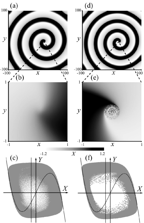
Figure 1: Spiral patterns exhibited by non-locally coupled FitzHugh-Nagumo oscillators for two representative cases of strong coupling ((a),(b) and (c), $K=10.0$) and weak coupling ((d),(e) and (f), $K=5.0$). Other parameters are fixed as $a=1.0$, $b=0.2$, $\sigma=0.1$ and $D=1$. (a) and (d): Overall patterns of the component $X$ displayed in gray scale. (b) and (e): Their structures near the core. (c) and (f): Corresponding phase portraits in the $X$-$Y$ plane, where the nullclines $f(X,Y)=0$ and $g(X,Y)=0$ are also indicated.

II.3 Estimation of $K_{c}$

From the numerical data presented in FIG. 1, one may expect the existence of a critical value of the coupling strength, denoted as $K_{c}$, associated with the onset of incoherence. We now try to estimate $K_{c}$ for our system of non-locally coupled FitzHugh-Nagumo oscillators given by Eqs. (1), (2), (5) and (7), where the spatial extension is supposed to be infinite. Consider first the situation where the coupling is large enough for the system to sustain a rigidly rotating spiral wave with sufficient spatial smoothness. The corresponding solution is represented by $\mbox{\boldmath$A$}_{s}(\mbox{\boldmath$r$},t)=(X_{s}(\mbox{\boldmath$r$},t),Y_{s}(\mbox{\boldmath$r$},t))$. Let the center of rotation be at $\mbox{\boldmath$r$}=0$. By assumption, the oscillator right at the center is motionless, i.e., $\mbox{\boldmath$A$}_{s}(0,t)=(X_{c},Y_{c})$, where $X_{c}$ and $Y_{c}$ are time-independent. Our question is at which value of $K$ this fixed point becomes unstable and the oscillator there starts to oscillate. To consider this problem, it is convenient to work with the aforementioned mean-field picture by which we look upon the local oscillators as being subject to a common space-time dependent field $B$. The mean field pattern should also rotate rigidly around $\mbox{\boldmath$r$}=0$, so that the central oscillator is subject to a constant forcing $B(0)$. The system of Eqs. (1) and (2) describing this particular oscillator form an autonomous two-dimensional dynamical system, so that once $B(0)$ is known the value of the fixed point $(X_{c},Y_{c})$ and its stability will easily be found. The value of $B(0)$ can actually be estimated from Eq. (5) by developing $X_{s}(\mbox{\boldmath$r$},t)$ into a Taylor series about $\mbox{\boldmath$r$}=0$, which is allowed owing to the assumed smoothness of the pattern. It is clear that, as a result of the isotropy of the coupling function $G$, there is no contribution to $B(0)$ from the first order expansion terms. If the contribution from the second order terms is negligible, i.e., if the nonlinear variation of $X_{s}$ within the coupling range about $\mbox{\boldmath$r$}=0$ is negligible, then we may simply put $B(0)=X_{c}$. With this approximation, it is clear from Eqs. (1) and (2) that the fixed point $(X_{c},Y_{c})$ is identical with the intersection of the nullclines $f=g=0$, i.e., the unstable fixed point of the local oscillators. Its linear stability is also easy to analyze. The result is that the critical coupling strength is given by $K_{c}=(1-3X_{c}^{2})/\sigma$ below which the fixed point $(X_{c},Y_{c})$ becomes Hopf unstable. Applying the values of $a$, $b$ and $\sigma$ used in our numerical simulations, we obtain $K_{c}=8.8$. This value of $K_{c}$ is consistent with our direct numerical simulation, although its precise numerical determination is yet unavailable.

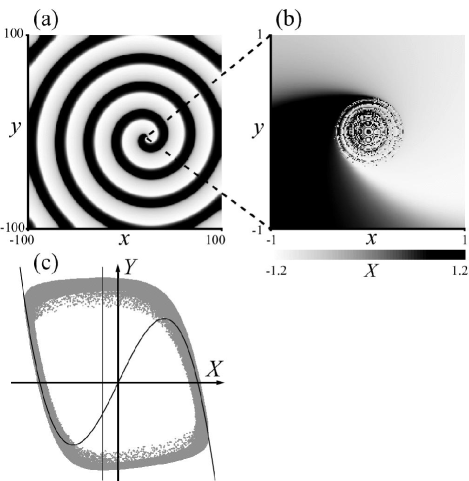
Figure 2: Spiral patterns exhibited by non-locally coupled FitzHugh-Nagumo oscillators with $K=2.0$, presented in a similar manner to FIG. 1. For this value of $K$, the amplitude degrees of freedom become almost irrelevant.

III SPIRAL DYNAMICS IN NON-LOCALLY COUPLED PHASE OSCILLATORS

In order to look into the nature and origin of our anomalous spiral dynamics in further detail, we now consider the situation where the coupling is much weaker than $K_{c}$. Figure 2 shows some results from our numerical simulation carried out for $K=2.0$, presented in a similar manner to FIG. 1. While there seems nothing unusual about the overall spiral pattern, the corresponding phase portrait forms a ring with a relatively thin periphery, which is totally unlike a simply connected object. We may alternatively say that the oscillator amplitude everywhere takes almost a full value. This is exactly the situation where the so-called phase description is applicable. In fact, as we see later in this section, a simple phase oscillator model with non-local coupling can develop a spiral pattern with phase-randomized core similar to the above.

We now present a brief review of the phase reduction methodKuramoto (1984) in the form appropriate for the present purposes. Each of our local oscillators without coupling is described by a two-dimensional dynamical system $d\mbox{\boldmath$A$}/dt=\mbox{\boldmath$F$}(\mbox{\boldmath$A$})$, where $\mbox{\boldmath$A$}=(X,Y)$ and $\mbox{\boldmath$F$}=(f,g)$. Let its stable time-periodic solution with frequency $\omega$ be given by $\mbox{\boldmath$A$}_{0}(\omega t)=(X_{0}(\omega t),Y_{0}(\omega t))$, which is a $2\pi$-periodic function of $\omega t$. The corresponding limit-cycle orbit is represented by $\cal C$. Phase $\phi$ associated with this oscillator must be defined outside $\cal C$ as well as on $\cal C$. Most conveniently, it is defined in such a way that the free motion of the oscillator satisfies $d\phi/dt=\omega$ regardless of initial conditions. This requires that $\phi$ as a scalar field $\phi(\mbox{\boldmath$A$})$ satisfies the identity $\mbox{grad}_{\boldsymbol{A}}\phi\cdot\mbox{\boldmath$F$}(\mbox{\boldmath$A$})=\omega$. The whole $X$-$Y$ plane is then filled with equi-phase lines which are called isochrons, one of which is chosen to correspond to the zero phase. Corresponding to each $\phi$-value, a point $\mbox{\boldmath$A$}_{0}(\phi)$ on $\cal C$ is determined uniquely, which says nothing but the fact that an isochron and $\cal C$ intersect at a single point.

When the non-local coupling is introduced, the equation for each local oscillator is modified as

$$\partial_{t}\mbox{\boldmath$A$}(\mbox{\boldmath$r$},t)=\mbox{\boldmath$F$}(\mbox{\boldmath$A$})+\mbox{\boldmath$p$}(\mbox{\boldmath$r$},t),$$ (8)

where

$$\mbox{\boldmath$p$}(\mbox{\boldmath$r$},t)=(p_{X}(\mbox{\boldmath$r$},t),0),$$

$$p_{X}(\mbox{\boldmath$r$},t)=K\int G(\mbox{\boldmath$r$}-\mbox{\boldmath$r$}^{\prime})\left[X(\mbox{\boldmath$r$}^{\prime},t)-X(\mbox{\boldmath$r$},t)\right]d\mbox{\boldmath$r$}^{\prime}.$$

Correspondingly, the equation for the phase is modified as

$$\partial_{t}\phi=\mbox{grad}_{\boldsymbol{A}}\phi\cdot(\mbox{\boldmath$F$}(\mbox{\boldmath$A$})+\mbox{\boldmath$p$})=\omega+\mbox{grad}_{\boldsymbol{A}}\phi\cdot\mbox{\boldmath$p$}.$$ (9)

If the perturbation $p$ is sufficiently weak, which we assume now, the oscillator will keep staying on $\cal C$ in good approximation. Then $\mbox{grad}_{\boldsymbol{A}}\phi$ in Eq. (9) may safely be evaluated on $\cal C$, or

$$\mbox{grad}_{\boldsymbol{A}}\phi\simeq(Z_{X}(\phi),Z_{Y}(\phi)),$$

where

$$Z_{X}(\phi)=[\partial_{X}\phi(\mbox{\boldmath$A$})]_{\boldsymbol{A}=\boldsymbol{A}_{0}(\phi)},$$

and $Z_{Y}(\phi)$ is defined similarly. At the same time, $p_{X}$ may be approximated with

$$p_{X}\simeq K\int G(\mbox{\boldmath$r$}-\mbox{\boldmath$r$}^{\prime})[X_{0}(\phi(\mbox{\boldmath$r$}^{\prime},t))-X_{0}(\phi(\mbox{\boldmath$r$},t))]d\mbox{\boldmath$r$}^{\prime}.$$

Thus, the phase equation becomes

$$\partial_{t}\phi(\mbox{\boldmath$r$},t) = \omega+KZ_{X}(\phi(\mbox{\boldmath$r$},t))$$

$$\times\int G(\mbox{\boldmath$r$}-\mbox{\boldmath$r$}^{\prime})[X_{0}(\phi(\mbox{\boldmath$r$}^{\prime},t))-X_{0}(\phi(\mbox{\boldmath$r$},t))]d\mbox{\boldmath$r$}^{\prime}.$$

Since the small effect of the perturbation on $\partial_{t}\phi$ can be time-averaged over one cycle of oscillationKuramoto (1984), the phase equation finally takes the form

$$\partial_{t}\phi(\mbox{\boldmath$r$},t)=\omega+K\int G(\mbox{\boldmath$r$}-\mbox{\boldmath$r$}^{\prime})\Gamma\big{(}\phi(\mbox{\boldmath$r$},t)-\phi(\mbox{\boldmath$r$}^{\prime},t)\big{)}d\mbox{\boldmath$r$}^{\prime},$$ (10)

where

$$\Gamma(\phi-\phi^{\prime})=\frac{1}{2\pi}\int_{0}^{2\pi}Z_{X}(\lambda+\phi)\left[X_{0}(\lambda+\phi^{\prime})-X_{0}(\lambda+\phi)\right]d\lambda.$$

By using the above formula, $\Gamma(\phi)$ may be computed numerically if the forms of $f$ and $g$ are given explicitly. For the present case of FitzHugh-Nagumo oscillators, numerically obtained $\Gamma(\phi)$ is displayed in FIG. 3.

The phase-coupling function $\Gamma(\phi)$, which is a $2\pi$-periodic function of $\phi$, generally involves various harmonics, and this is also true of the curve given in FIG. 3. We still expect that the spiral dynamics of our concern does not depend so heavily on the specific form of $\Gamma(\phi)$. Therefore, in order for further mathematical analysis to be practicable, we will work with a simplest in-phase type coupling function, i.e., $\Gamma(\phi)=-\sin(\phi+\alpha)$ ($|\alpha|<\pi/2$). Thus, the phase equation takes the form

$$\partial_{t}\phi(\mbox{\boldmath$r$},t)=\omega-K\int G(\mbox{\boldmath$r$}-\mbox{\boldmath$r$}^{\prime})\sin\big{(}\phi(\mbox{\boldmath$r$},t)-\phi(\mbox{\boldmath$r$}^{\prime},t)+\alpha\big{)}d\mbox{\boldmath$r$}^{\prime}$$ (11)

for which an in-depth mathematical analysis is possible as we see below.

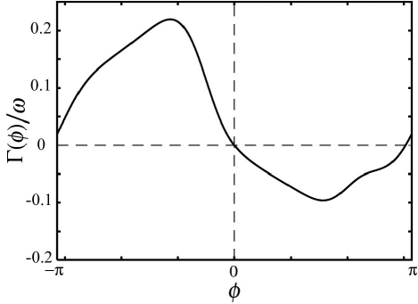
Figure 3: Phase-coupling function $\Gamma(\phi)$ versus $\phi$ for coupled FitzHugh-Nagumo oscillators. This quantity can be used for the study of non-locally coupled phase oscillators given by Eq. (10).

Before proceeding to the analysis of Eq. (11), we remark that the above phase equation is also a correct reduced form of a non-local version of the complex Ginzburg-Landau equationTanaka , the latter itself being a reduced form of our three-component reaction-diffusion model close to the Hopf bifurcation and comparably close to the limit of vanishing couplingTanaka and Kuramoto (2003). This fact gives a further support to our view that the application of Eq. (11) to our problem is reasonable.

We are still far from a full understanding of the solution to the universal equation (11), and our concern below is its spiral wave solution in two dimensions. Although the equation involves four parameters $\omega$, $K$, $r_{0}$ and $\alpha$, the only relevant parameter is $\alpha$. The reason is the following. Firstly, $r_{0}$, on which $G(r)$ depends (see Eq. (6)), may be chosen to be the length unit, so that we may put $r_{0}=1$. Similarly, the coupling strength $K$ may be fixed to 1 by suitably choosing the time unit. The natural frequency $\omega$ can be eliminated by working with a suitable co-moving frame of reference, i.e., via the transformation $\phi\rightarrow\phi+\omega t$. In the following analysis, however, the irrelevant parameter $\omega$ is retained as a nonzero constant, while we choose $\alpha=0.3$ and $r_{0}=K=1$.

Numerical simulation of Eq. (11) was carried out in a two-dimensional system. The numerical scheme adopted is the same as that explained in the previous section. As expected, we see from FIG. 4 the appearance of rotating spiral waves with a disordered group of oscillators near the core very similar to what we have seen in the previous section.

For the arguments developed below, it is convenient to define a mean field $W(\mbox{\boldmath$r$},t)$ through

$$W(\mbox{\boldmath$r$},t)=\int G(\mbox{\boldmath$r$}-\mbox{\boldmath$r$}^{\prime})\exp[i\phi(\mbox{\boldmath$r$}^{\prime},t)]d\mbox{\boldmath$r$}^{\prime}.$$ (12)

The modulus $R$ and the phase $\Theta$ of this complex quantity are defined by

$$W(\mbox{\boldmath$r$},t)=R(\mbox{\boldmath$r$},t)\exp[i\Theta(\mbox{\boldmath$r$},t)].$$

Since the definition (12) of the mean field involves a weighted spatial average over infinitely many local oscillators, this quantity is expected to be smooth in space even these oscillators are behaving incoherently. This property of $W$ is also clear from the differential form of Eq. (12), i.e.,

$$0=-W+\nabla^{2}W+\exp(i\phi).$$ (13)

The above equation implies a strong similarity of $W$ to $B$ governed by Eq. (4). If the mean field pattern rotates steadily with frequency $\Omega$, then $R$ is time-independent and the relative mean field phase $\Theta_{0}$ defined by

$$\Theta(\mbox{\boldmath$r$},t)=\Omega t+\Theta_{0}(\mbox{\boldmath$r$},t)$$

is also time-independent.

In terms of $R(\mbox{\boldmath$r$},t)$ and $\Theta(\mbox{\boldmath$r$},t)$, Eq. (11) may be expressed in the form of a one-oscillator dynamics

$$\partial_{t}\phi(\mbox{\boldmath$r$},t)=\omega-R(\mbox{\boldmath$r$},t)\sin\big{(}\phi(\mbox{\boldmath$r$},t)+\alpha-\Theta(\mbox{\boldmath$r$},t)\big{)},$$

or if we introduce a relative phase variable $\psi(\mbox{\boldmath$r$},t)$ through

$$\phi(\mbox{\boldmath$r$},t)=\Omega t+\psi(\mbox{\boldmath$r$},t),$$

we have

$$\partial_{t}\psi(\mbox{\boldmath$r$},t)=\omega-\Omega-R(\mbox{\boldmath$r$},t)\sin\big{(}\psi(\mbox{\boldmath$r$},t)+\alpha-\Theta_{0}(\mbox{\boldmath$r$},t)\big{)}.$$ (14)

The definition of the mean field given by Eq. (12) becomes

$$R(\mbox{\boldmath$r$},t)\exp[i\Theta_{0}(\mbox{\boldmath$r$},t)]=\int G(\mbox{\boldmath$r$}-\mbox{\boldmath$r$}^{\prime})\exp[i\psi(\mbox{\boldmath$r$}^{\prime},t)]d\mbox{\boldmath$r$}^{\prime}.$$ (15)

Note that the set of Eqs. (14) and (15) is still equivalent to the original phase equation (11).

We now proceed to some anatomy of the anomalous core structure taking advantage of the numerically observed fact that the mean field pattern has a well-defined center of rotation (chosen to be $\mbox{\boldmath$r$}=0$) at which $W=0$. One may thus imagine a linear cross section $\cal S$ of the pattern passing through $\mbox{\boldmath$r$}=0$ and study the radial profiles of various quantities emerging along $\cal S$. Some results obtained in this way of analysis are summarized in FIG. 5 (a) to (c).

An instantaneous radial profile of the mean field modulus $R$ is presented in FIG. 5 (a). As expected, it has a vanishing value at the origin, and its temporal fluctuation is also found negligibly small.

Figure 5 (b) shows an instantaneous distribution of the phases $\phi$ of the local oscillators lying on $\cal S$ (indicated by crosses ). The same panel also includes the pattern of the mean field phase $\Theta$ on the same cross section (indicated by open circles). It is clear that there exists a well-defined critical radius separating the domains of coherent and incoherent oscillators from each other. We also confirmed (but not shown explicitly) that the profiles of the mean field phase and that of the phases of the coherent oscillators are almost stationary except for a vertical drift with constant velocity $\Omega$.

Our interpretation of the results given by FIGs. 5 (a) and (b) is that the entire system now splits into two subdomains such that the oscillators in one domain synchronize completely with the periodic mean-field forcing, while those in the other domain fail in synchronization. Further evidence supporting this interpretation is provided in FIG. 5 (c) where the distribution of the mean frequency $\bar{\omega}$ (defined by a long-time average of $\partial_{t}\phi$) of the local oscillators lying on $\cal S$ is shown. This frequency pattern is clearly composed of two parts. Namely, in the outer domain the oscillators have an identical frequency, while in the inner domain the frequencies are distributed, the latter implying phase randomization consistent with the scattered dots appearing in FIG. 5 (b).

In the next section, we develop a theory for determining the mean field pattern together with its rotation frequency, and also the motion of the individual oscillators driven by this mean field, in a self-consistent manner.

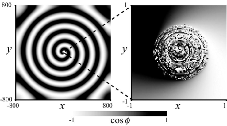
Figure 4: Spiral pattern (left) and its core structure (right) exhibited by non-locally coupled phase oscillators governed by Eq. (11), where $\alpha=0.3$.

IV THEORY

The basic equations to work with are Eqs. (14) and (15). Our theory starts with the assumption that the mean-field pattern is steadily rotating, and therefore we drop the $t$-dependence from $R$ and $\Theta_{0}$ in these equations. A complete solution to this system of equations can be obtained in the following two steps. We first solve Eq. (14) for each $\psi$ as a function of $R$ and $\Theta_{0}$, which is easy to do. Note that $R$ and $\Theta_{0}$ are the quantities yet to be determined. Secondly, the entire set of these solutions is substituted into Eq. (15). The right-hand side of Eq. (15) thus becomes a functional of the mean field. In this way, the mean field value at each spatial point is expressed in terms of a functional of the mean field itself. Solution of this functional self-consistency equation exists only for a special value of the rotation frequency $\Omega$ of the mean field pattern. We will therefore be working with a non-linear eigenvalue problem. The final solution of this functional equation could be found only numerically.

The above self-consistent way of finding a solution to a many-oscillator problem resembles strongly Kuramoto’s 1975 theory of synchronization phase transition in a large population of globally coupled oscillators with distributed natural frequenciesKuramoto (1975). The main difference is that the oscillators are now coupled non-locally rather than globally, and consequently the mean field is generally space-dependent leading to a functional self-consistency equation rather than a simple transcendental equation. Although the natural frequencies of the oscillators are identical in the present case, the actual frequencies can be distributed due to the existence of a spatial gradient of the mean field. A simpler, one-dimensional version of the present type of theory based on a similar model of non-locally coupled phase oscillators was reported earlierKuramoto and Battogtokh (2002).

An important feature common to all such theories is that the one-oscillator equation which involves the mean field amplitude as a parameter admits either a stationary solution or a drifting solution. Which one to hold depends on the modulus of the mean-field. The crucial point to the theory is how to deal with the drifting solutions, because a simple substitution of this type of solutions into the definition of the mean field apparently contradicts the assumed stationarity of the mean field (in a suitable co-moving frame of reference). The seeming contradiction here can be resolved by using the invariant measure associated with the drift motion. We will now show explicitly the steps leading to an exact solution to the problem.

As stated above, there are two possible cases regarding the solution of Eq. (14).

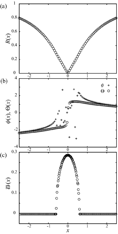
Figure 5: Radial profiles of various quantities corresponding to the spiral core of FIG. 4. (a) Instantaneous radial profile of the mean-field modulus $R$. (b) Instantaneous radial profile of the phases $\phi$ of the local oscillators (crosses) and that of the mean field phase $\Theta$ (open circles). (c) Radial profile of the mean frequency $\bar{\omega}$ (defined by a long-time average of $\partial_{t}\phi$) of the local oscillators.

They are: (Case I) $|\omega-\Omega|<R$, and (Case II) $|\omega-\Omega|>R$. Correspondingly, the oscillators are divided into two groups. In the first case, which corresponds to the group of coherent oscillators, Eq. (14) admits a pair of stable and unstable fixed points. The stable one, denoted by $\psi_{0}(\mbox{\boldmath$r$})$, is given by

$$\psi_{0}(\mbox{\boldmath$r$})=\mbox{Sin}^{-1}\Biggl{(}\frac{\omega-\Omega}{R(\mbox{\boldmath$r$})}\Biggr{)}+\Theta_{0}(\mbox{\boldmath$r$})-\alpha.$$

The actual frequencies $\bar{\omega}$ of the oscillators in this group are of course identical with $\Omega$. We substitute the above solution for $\psi(\mbox{\boldmath$r$})$ into Eq. (15), and restrict the integral to the domain where the inequality $|\omega-\Omega|<R(\mbox{\boldmath$r$})$ is satisfied. In this way, the contribution to the local mean field value coming from the coherent group of oscillators is obtained.

The second case corresponds to the group of incoherent oscillators, for which Eq. (14) admits a drifting solution. The actual frequencies $\bar{\omega}(\mbox{\boldmath$r$})$ are now distributed and they are easily calculated as

$$\begin{split}\bar{\omega}&=\Omega+2\pi\Big{[}\int_{0}^{2\pi}\Big{(}\frac{d\psi}{dt}\Big{)}^{-1}d\psi\Big{]}^{-1}\\ &=\Omega+(\omega-\Omega)\sqrt{1-\left(\frac{R}{\omega-\Omega}\right)^{2}}.\end{split}$$

The contribution to the local mean field value from this incoherent group of oscillators can be found in the following way. Since $\psi$ is drifting, the factor $\exp(i\psi)$ in the integrand in Eq. (15) does not have a definite value. We are thus led to the idea that this factor should rather be replaced with its statistical average which can be calculated by using the invariant measure, i.e., the probability density $p(\psi)$ associated with the drift motion. Noting that the probability density for the oscillator’s phase to take on value $\psi$ must be inversely proportional to the drift velocity given by the right-hand side of Eq. (14), we have

$$p(\psi)=C\left[\omega-\Omega-R\sin\big{(}\psi+\alpha-\Theta_{0}\big{)}\right]^{-1},$$ (16)

where $C$ is the normalization constant given by $C=(2\pi)^{-1}(\omega-\Omega)\sqrt{1-R^{2}/(\omega-\Omega)^{2}}$.

Putting together the above-stated two types of contributions to the mean field, we finally obtain a functional self-consistency equation in the form

$$R(\mbox{\boldmath$r$})e^{i\Theta_{0}(\mbox{\boldmath$r$})}=\int G(\mbox{\boldmath$r$}-\mbox{\boldmath$r$}^{\prime})h(R(\mbox{\boldmath$r$}^{\prime}),\Theta_{0}(\mbox{\boldmath$r$}^{\prime}),\omega-\Omega)d\mbox{\boldmath$r$}^{\prime},$$ (17)

where

$$h(R,\Theta_{0},\omega-\Omega)=\begin{cases}\exp[i\psi_{0}(R,\Theta_{0},\omega-\Omega)]\\ \qquad\qquad\qquad\qquad\quad(\lvert\omega-\Omega\rvert<R),\\ \int_{-\pi}^{\pi}p(\psi,R,\Theta_{0},\omega-\Omega)\exp(i\psi)d\psi\\ \qquad\qquad\qquad\qquad\quad(\lvert\omega-\Omega\rvert>R),\end{cases}$$

or more explicitly

$$e^{i\psi_{0}}=e^{i(\Theta_{0}-\alpha)}\left\{\sqrt{1-\left(\frac{\omega-\Omega}{R}\right)^{2}}+i\frac{\omega-\Omega}{R}\right\},$$

$$\int_{-\pi}^{\pi}p(\psi)e^{i\psi}d\psi = ie^{i(\Theta_{0}-\alpha)}\left(\frac{\omega-\Omega}{R}\right)$$

$$\times\left\{1-\sqrt{1-\left(\frac{R}{\omega-\Omega}\right)^{2}}\right\}.$$

Numerical solution of Eq. (17) can be found iteratively. We did this in a finite domain defined by $x,y\in[0,40]$ with $G$ appropriate for the free boundary conditions imposed on Eq. (13). Since a solution of Eq. (17) would only be available for a special value of $\Omega-\omega$ which is still to be determined, its trial value was adjusted in each iteration step in such a way that a suitably defined distance between the two mean-field patterns, one produced at the current step and the other at the next step, may be minimized. In this way, by starting with a suitable initial mean field pattern similar to the one obtained from numerical simulations, a rapid convergence of the mean field pattern and the value of $\Omega$ was achieved.

In FIG. 6 our theoretical results obtained in this way are compared with the data given in FIG. 5, i.e., the results from direct numerical simulation of Eq. (11). The agreement is so excellent that our theory is expected to hold exactly in the continuum limit.

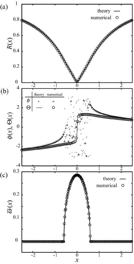
Figure 6: Comparison between the theory and numerical simulation. Theoretical results are indicated with solid lines in (a) and (c), and solid lines and scattered dots in (b). Numerical data, which are the same as those given in FIG. 5, are indicated with open circles and crosses. (a) Instantaneous radial profile of the mean-field modulus $R$. (b) Instantaneous radial profile of the mean-field phase $\Theta$, and that of the phases $\phi$ of the local oscillators, where the theoretically obtained scattered dots are the random numbers chosen from the probability distribution given by Eq. (16). (c) Radial profile of the mean frequency $\bar{\omega}$ of the local oscillators.

V SUMMARY AND CONCLUDING REMARKS

Spontaneous generation of a local group of phase-randomized oscillators near the center of a rotating spiral pattern was confirmed through numerical simulations on non-locally coupled oscillators. It was argued that smaller value of the coupling strength favors the occurrence of the core anomaly. The critical coupling strength $K_{c}$ associated with the onset of this anomaly was estimated from a simple argument. When $K$ is sufficiently small, by which the oscillation amplitude even near the center of rotation takes almost a full value, a group of incoherent oscillators always exists. Still the overall spiral pattern looks completely normal. Guided by this fact observed numerically, we applied the phase reduction method for the purpose of gaining a deeper understanding of the phenomenon. The resulting phase oscillator model with non-local coupling was found to exhibit the same type of core anomaly. Under the assumption that the pattern of a suitably defined mean field is steadily rotating in spite of the existence of incoherence, we derived a functional self-consistency equation to be satisfied by the mean field. Its solution successfully reproduced various results obtained from our direct numerical simulations carried out on this phase model.

Finally, we remark that the present study is confined to a particular domain of parameter values where the mean field dynamics is regular. Our preliminary study suggests that under different conditions more complex collective dynamics occurs, which is characterized, e.g., by an elongation of the domain of incoherent oscillators and its irregular motionKuramoto and Shima (2003). For the case of non-locally coupled FitzHugh-Nagumo oscillators for small $K$, this occurs for larger $b$, i.e., when the symmetry of the local oscillator dynamics is lowered, although a perfect symmetry ($b=0$, or the van der Pol limit) is not necessary for the steady rotation of the mean field. For larger $K$ (still below $K_{c}$), in contrast, regular dynamics of the mean field and circular shape of the domain of incoherent oscillators seem to persist against relatively strong asymmetry of the oscillator dynamics. These results will be reported elsewhere.