On computational irreducibility and the predictability of complex physical systems

Abstract

Using elementary cellular automata (CA) as an example, we show how to coarse-grain CA in all classes of Wolfram’s classification. We find that computationally irreducible (CIR) physical processes can be predictable and even computationally reducible at a coarse-grained level of description. The resulting coarse-grained CA which we construct emulate the large-scale behavior of the original systems without accounting for small-scale details. At least one of the CA that can be coarse-grained is irreducible and known to be a universal Turing machine.

Can one predict the future evolution of a physical process which is described or modeled by a computationally irreducible (CIR) mathematical algorithm? For such systems, in order to know the system’s state after (e.g.) one million time steps, there is no faster algorithm than to solve the equation of motion a million time steps into the future. Wolfram has suggested that the existence of CIR systems in nature is at the root of our apparent inability to model and understand complex systems Wolfram (1984a, 1985, 2002); Ilachinski (2001).

Complex physical systems that are CIR might therefore seem to be inherently unpredictable. It is tempting to conclude from this that the enterprise of physics itself is doomed from the outset; rather than attempting to construct solvable mathematical models of physical processes, computational models should be built, explored and empirically analyzed. This argument, however, assumes that infinite precision is required for the prediction of future evolution. Usually coarse-grained or even statistical information is sufficient: indeed, a physical model is usually correct only to a certain level of resolution, so that there is little interest in predictions from such a model on a scale outside its regime of validity.

In this Letter, we report on experiments with nearest neighbour one-dimensional cellular automata, which show that because in practice one only seeks coarse-grained information, complex physical systems can be predictable and even computationally reducible at some level of description. The implication of these results is that, at least for systems whose complexity is the outcome of very simple rules, useful approximations can be made that enable predictions about future behavior.

Cellular automata (CA) are dynamical systems composed of a lattice of cells. Each cell in the lattice can assume a value from a given finite alphabet. The system evolves in time according to an update rule that gives a cell’s new state as a function of values in its finite neighborhood. CA were originally introduced by von Neumann and Ulam von Neumann (1966) in the 1940’s as a possible way of simulating self reproduction in biological systems. Since then, CA have attracted a great deal of interest in physics Wolfram (1983); phy ; Ilachinski (2001); Wolfram (1994) because they capture two basic ingredients of many physical systems: 1) they evolve according to a local uniform rule. 2) CA can exhibit rich behavior even with very simple update rules. For similar and other reasons, CA have also attracted attention in computer science Mitchel (1998); Sarkar (2000), biology Ermentrout and Edelstein-Keshet (1993), material science Raabe (2002) and other fields.

In early work Wolfram (1984b, a, 1985, 2002), Wolfram proposed that CA can be grouped into four classes of complexity. Class 1 consists of CA whose dynamics reaches a steady state regardless of the initial conditions. Class 2 consists of CA whose long time evolution produces periodic or nested structures. CA from both of these classes are simple in the sense that their long time evolution can be deduced from running the system a small number of time steps. On the other hand, class 3 and class 4 consist of “complex” CA. Class 3 CA produce structures that seem random. Class 4 CA produce a mixture of random structures and periodic behavior. This transition in CA complexity was later regarded as a phase transitionLangton (1990) in the CA rule space. For a review on CA classification see Refs. Mitchel, 1998; Ilachinski, 2001; Wolfram, 2002. There is no generally agreed upon algorithm for classifying a given CA. The assignment of CA to these four classes is somewhat subjective and, we will argue, may need to be refined. Based on numerical experiments, Wolfram hypothesized Wolfram (1984b, a, 2002) that most CA from class 3 and 4 are CIR.

There is no unique way to define coarse-graining, but here we will mean that our information about the CA is locally coarse-grained in the sense of being stroboscopic in time, but that nearby cells are grouped into a supercell according to some specified rule (as is frequently done in statistical physics). A system which can be coarse-grained is compactable since it is possible to calculate its future time evolution (or some coarse aspects of it) using a more compact algorithm than its native description. Note that our use of the term compactable refers to the phase space reduction associated with coarse-graining, and is agnostic as to whether or not the coarse-grained system is reducible or irreducible. Accordingly, we define predictable to mean that a system is computationally reducible or has a computationally reducible coarse-graining. Thus, it is possible to calculate the future time evolution of a predictable system (or some coarse aspects of it) using an algorithm which is more compact than both the native and coarse-grained descriptions.

In order to quantify the implications of looking at coarse-grained information only, we have systematically attempted to coarse-grain the 256 nearest neighbor one-dimensional binary CA that were the subject of Wolfram’s investigationsWolfram (2002, 1983). The outcome, described in detail below, is surprising: we found that many CA can be coarse-grained and that in some cases CIR CA are coarse-grained by computationally reducible ones. In other words, even though microscopically a given system might be CIR, its coarse-grained dynamics can be compactable and predictable.

We start by defining a simple procedure for coarse-graining a CA. Other constructions are undoubtedly possible. For simplicity we limit our treatment to one-dimensional systems with nearest neighbor interactions. Generalizations to higher dimensions and different interaction radii are straightforward. Let $A=\left(a\left(t\right),S_{A},f_{A}\right)$ be a cellular automaton defined on an array of cells $a\left(t\right)=\left.\left\{a_{n}\left(t\right)\right\}\right|_{n=-\infty}^{\infty}$. Each cell accepts an alphabet of $S_{A}$ symbols, namely $a_{n}\left(t\right)\in\left\{0\dots S_{A}-1\right\}$. The values of the cells evolve in time according to the update rule $a_{n}\left(t+1\right)=f_{A}\left[a_{n-1}\left(t\right),a_{n}\left(t\right),a_{n+1}\left(t\right)\right]$, where $f_{A}:\left\{S_{A}\right\}^{3}\rightarrow\left\{S_{A}\right\}$ is the transition function. The update rule is applied simultaneously to all the cells and we denote this application by $a\left(t+1\right)=f_{A}\cdot a\left(t\right)$.

Our goal is to find a modified CA $B=\left(b\left(t\right),S_{B},f_{B}\right)$ and an irreversible coarse-graining function $b=C\left(a\right)$, which are capable of a coarse-grained emulation of $A$. For every initial condition $a(0)$, $B$ and $C$ must satisfy:

$$C\left(f_{A}^{T\cdot t}\cdot a(0)\right)=f_{B}^{t}\cdot C\left(a(0)\right).$$ (1)

Namely, running the original CA for $T\cdot t$ time steps and then coarse-graining is equivalent to coarse-graining the initial condition and then running the modified CA $t$ time steps. The constant $T$ is a time scale associated with the coarse-graining.

To search for explicit coarse-graining rules, we define the $N$’th block version $A^{N}=\left(a^{N},S_{A^{N}},f_{A^{N}}\right)$ of $A$. $S_{A^{N}}=\left(S_{A}\right)^{N}$ and each cell in $A^{N}$ represents a block of $N$ cells in $A$. Cell values are translated between $A$ and $A^{N}$ according to the base $S_{A}$ value of $N$ cells in $A$. The transition function $f_{A^{N}}:\left\{S_{A^{N}}\right\}^{3}\rightarrow\left\{S_{A^{N}}\right\}$ is computed by running $A$ for $N$ time steps on all possible initial conditions of length $3N$. In this way $A^{N}$ computes in one time step $N$ time steps of $A$. Note that $A^{N}$ is not a coarse-graining of $A$ because no information was lost in the cell translation.

Next we attempt to generate the coarse CA $B$ by projecting the alphabet of $A^{N}$ on a subset of $\left\{0\dots S_{A^{N}}-1\right\}$. This is the key step where information is being lost, a manipulation which distinguishes between coarse-graining and emulation blocking transformations Wolfram (2002); Ilachinski (2001). The transition function $f_{B}$ is constructed from $f_{A^{N}}$ by projecting its arguments and outcome:

$$f_{B}\left[\overline{x_{1}},\overline{x_{2}},\overline{x_{3}}\right]=\overline{f_{A^{N}}\left[\overline{x_{1}},\overline{x_{2}},\overline{x_{3}}\right]}.$$ (2)

Here $\overline{x}\equiv P\left(x\right)$ denotes the projection operation. This construction is possible only if

$$\overline{f_{A^{N}}\left[x_{1},x_{2},x_{3}\right]}=\overline{f_{A^{N}}\left[y_{1},y_{2},y_{3}\right]},\;\;\forall\left(x,y|\overline{x_{i}}=\overline{y_{i}}\right).$$ (3)

Otherwise, $f_{B}$ is multi-valued and our coarse-graining attempt fails for the specific choice of $N$ and $P$.

In cases where the above conditions are satisfied, the resulting CA $B$ is a coarse-graining of $A^{N}$ with a time scale $T=1$. For every step $a^{N}_{n}(t+1)=f_{A^{N}}\left[a^{N}_{n-1}(t),a^{N}_{n}(t),a^{N}_{n+1}(t)\right]$ of $A^{N}$, $B$ makes the move

$$b_{n}(t+1) = f_{B}\left[b_{n-1}(t),b_{n}(t),b_{n+1}(t)\right]$$

$$= \overline{f_{A^{N}}\left[\overline{a^{N}_{n-1}(t)},\overline{a^{N}_{n}(t)},\overline{a^{N}_{n+1}(t)}\right]}=\overline{a^{N}_{n}(t+1)}\;,$$

where we have used Eq. (3) in the last step. $B$ therefore satisfies Eq. (1) with $P$ as the coarse-graining function. Since a single time step of $A^{N}$ computes $N$ time steps of $A$, $B$ is also a coarse-graining of $A$ with a coarse-grained time scale $T=N$. The coarse-graining function $C$ in this case is composed of the translation from $A$ to $A^{N}$ followed by the projection operator $P$. Analogies of these operators have been used in attempts to reduce the computational complexity of certain stochastic partial differential equations Hou et al. (2001); Degenhard and Rodriguez-Laguna (2002). Similar ideas have been used to calculate critical exponents in probabilistic CA de Oliveira and Satulovsky (1997); Monetti and Satulovsky (1998).

It is interesting to notice that the above coarse-graining procedure can lose two very different types of dynamic information. To see this, consider Eq. (3). This equation can be satisfied in two ways. In the first case

$$f_{A^{N}}\left[x_{1},x_{2},x_{3}\right]=f_{A^{N}}\left[y_{1},y_{2},y_{3}\right],\;\;\forall\left(x,y|\overline{x_{i}}=\overline{y_{i}}\right)\;,$$ (5)

which necessarily leads to Eq.  (3). $f_{A^{N}}$ in this case is insensitive to the projection of its arguments. The distinction between two variables which are identical under projection is therefore irrelevant to the dynamics of $A^{N}$, and by construction to the long time dynamics of $A$. By eliminating irrelevant degrees of freedom (DOF), coarse-graining of this type removes information which is redundant on the microscopic scale. The coarse CA in this case accounts for all possible long time trajectories of the original CA and the complexity classification of the two CA is therefore the same.

In the second case Eq. (3) is satisfied even though Eq. (5) is violated. Here the distinction between two variables which are identical under projection is relevant to the dynamics of $A$. Replacing $x$ by $y$ in the initial condition may give rise to a difference in the dynamics of $A$. Moreover, the difference can be (and in many occasions is) unbounded in space and time. Coarse-graining in this case is possible because the difference is constrained in the symbol space by the projection operator. Namely, projection of all such different dynamics results in the same coarse-grained behavior. Note that the coarse CA in this case cannot account for all possible long time trajectories of the original one. It is therefore possible for the original and coarse CA to fall into different complexity classifications.

Coarse-graining by elimination of relevant DOF removes information which is not redundant with respect to the original system. The information becomes redundant only when moving to the coarse scale. In fact, “redundant” becomes a subjective qualifier here since it depends on our choice of coarse description. In other words, it depends on what aspects of the microscopic dynamics we want the coarse CA to capture. In a sense, this is analogous to the subtleties encountered in constructing renormalization group transformations for the critical behavior of antiferromagnets Goldenfeld (1992); van Leeuwen (1975).

We now give specific examples of coarse-graining CA. In the sequel, CA rules are numbered using Wolfram’s notationWolfram (1983, 2002). Figure 1 (a) and (b) shows a coarse-graining of rule 146 by rule 128. Rule 146 produces a complex, seemingly random behavior which falls into the class 3 group. We use a super-cell size $N=3$, and project the alphabet $\{0\dots 7\}$ of the super-cells back to the $\{0,1\}$ alphabet with $P(7)=1$ and $P(x\neq 7)=0$pro . A triplet of cells in rule 146 are therefore coarse-grained to a single cell and the value of the coarse cell is $1$ only when the triplet are all $1$. Using this projection operator we construct the transition function of the coarse CA which is found to be rule 128, a class 1 CA. This choice of coarse-graining eliminates the small scale details of rule 146. Only structures of lateral size of three or more cells are accounted for. The decay of such structure in rule 146 is accurately described by rule 128.

Note that a class 3 CA was coarse-grained to a class 1 CA in the above example. Our gain was therefore two-fold. In addition to the phase space reduction associated with coarse-graining we have also achieved a reduction in complexity. Our procedure found predictable coarse-grained aspects of the dynamics even though the small scale behavior of rule 146 is complex, potentially CIR. As we explained earlier, this type of simplification can be achieved only by eliminating relevant DOF.

As a second example we show a transition between rules with a comparable complexity. Fig. 1 (c) and (d) shows a coarse-graining of rule 105 by rule 150. $N=2$ in this example and $P(x)=1$ only when $x=0,3$pro .

 

 

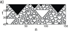
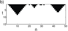
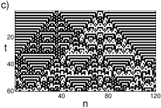
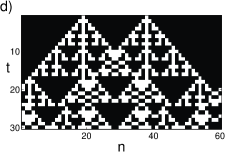
Figure 1: Examples of coarse-graining transitions. (a) and (b) show coarse-graining rule 146 by rule 128. (a) shows results of running rule 146. The top line is the initial condition and time progress from top to bottom. (b) shows the results of running rule 128 with the coarse grained initial condition from (a). (c) and (d) show coarse-graining rule 105 by rule 150. (c) shows rule 105 and (d) shows rule 150.

The coarse-graining procedure we described above is not constructive, but instead is a self-consistency condition on a putative coarse-graining rule with a specific block size $N$ and projection operator $P$. In many cases the coarse-graining fails and one must try other choices of $N$ and $P$. Can all CA be coarse-grained? If not, which CA can be coarse-grained and which cannot?

To answer these questions we tried systematically to coarse-grain Wolfram’s 256 elementary rules. We applied the coarse-graining procedure to each rule and scaned the $N$,$P$ space for valid solutions. In this way we were able to coarse-grain 240 out of the 256 CA dif . These 240 coarsen-able rules include members of all four classes. Many elementary CA can be coarse-grained by other elementary CA. Figure 2 shows a map of the coarse-graining transitions that we found within the family of elementary rules. Only coarse-grainings with $N\leq 4$ are shown due to limited computing power. Other transitions may exist with larger $N$. We observe that rule complexity never increases along the map’s transitions, i.e., coarse-graining introduces (at least here) partial order among CA rules.

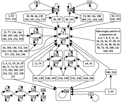
Figure 2: Coarse-graining transitions within the family of 256 elementary CA. Only transitions with a cell block size $N=2,3,4$ are shown. An arrow indicates that the origin rules can be coarse-grained by the target rules and may correspond to several choices of $N$ and $P$.

As mentioned above, we were unable to coarse-grain 16 elementary rules. 12 out of the 16 are the class 3 rules 30,45,106 and their symmetries. The other four are the class 2 rule 154 and it’s symmetries. We don’t know if our inability to coarse-grain these 16 rules comes from limited computing power or from something deeper.

It is worth noticing that a subset of the fixed points in the transition map is composed of all elementary additive rules (see page 952 in Ref. Wolfram, 2002) and their symmetries. This result is not limited to elementary rules. All additive CA whose alphabet sizes $S$ are prime numbers coarse-grain themselves with $N=S$ and $P$ the modulo $S$ sum of $S$ cells. We conjecture that there are situations where reducible fixed points exist for a wide range of systems, analogous to the emergence of amplitude equations in the vicinity of bifurcations points.

Coarse-graining transitions can also exit the elementary CA family. This happens whenever the alphabet of the coarse CA consists of more than two symbols. One such example which is of special importance is rule 110. Rule 110 is interesting because this class 4 CA is universal Wolfram (2002) in the Turing sense Herken (1995) and is therefore CIR Wolfram (1984b). It is capable of emulating all computations done by other computing devices in general and CA in particular.

We found several ways to coarse-grain rule 110. Using $N=6$, it is possible to project the 64 possible states onto an alphabet of 63 symbols. A more impressive reduction in the alphabet size is obtained by going to larger values of $N$. For $N=7,8,9,10,11$ we found an alphabet reduction of $6/128$, $22/256$, $67/512$, $181/1024$ and $463/2048$ respectively. We expect this behavior to persist for larger values of $N$.

Another interesting coarse-graining of rule 110 that we found is the transition to rule 0. Rule 0 has the trivial dynamics where all initial states evolve to the null configuration in a single time step. The transition to rule 0 is possible because the cell combination “01010” is not generated by rule 110 and can only appear in the initial state. Coarse-graining by rule 0 is achieved using $N=5$ and projecting “01010” to 1 and all other five cell combinations to 0. This example is important because it shows that even though rule 110 is CIR it has a predictable coarse-grained dynamics (however trivial). To our knowledge rule 110 is the only proven CIR elementary CA and therefore this is the only example of irreducible to reducible transition between elementary rules that we found.

We did find other complex, potentially CIR rules that can be coarse-grained by reducible CA. Rules 18, 54, 126 and their symmetries are coarse-grained by rule 0. As we showed above, rule 146 and it’s symmetries can be coarse-grained by rule 128 in a non-trivial way. We don’t know if these rules are CIR for lack of proof. Nevertheless, non-trivial irreducible to reducible transitions can in principle exist. Consider for example the CIR CA generated by the product of rules 110 and 128. Let the CA alphabet be $\{a,b\}\times\{0,1\}$, where the letters evolve according to rule 110 and the digits according to 128. We can recover the reducible, coarse-grain-able rule 128 by projecting the alphabet onto $\{0,1\}$.

The fact that CIR rules can be coarse-grained and that they has predictable coarse-grained dynamics shows that CIR is not a good measure of physical complexity. As in the case of rule 110, a CIR system may still yield an efficient predictable theory, provided that we are willing to ask coarse-grained questions. It seems that a better classification of physical complexity is related to what classes of projection operator are required to coarse-grain the system: local, real space projections or more complex non-geometric projections?

In summary, we have found that many CA, including CIR ones can be locally coarse-grained in space and time. In some cases CIR systems are predictable, if coarse-grained information only is required.

NG wishes to thank Stephen Wolfram for useful discussions and correspondence. This work was partially supported by the National Science Foundation through grant NSF-DMR-99-70690 (NG) and by the National Aeronautics and Space Administration through grant NAG8-1657.

References

- Wolfram (1984a) S. Wolfram, Nature 311, 419 (1984a).
- Wolfram (1985) S. Wolfram, Phys. Rev. Lett 54, 735 (1985).
- Wolfram (2002) S. Wolfram, A New Kind of Science (Wolfram media, Champaign, Ill., 2002).
- Ilachinski (2001) A. Ilachinski, Cellular Automata a Discrete Universe (World Scientific, Singapore, 2001).
- von Neumann (1966) J. von Neumann, Theory of Self-Reproducing Automata (University of Illinois Press, Urbana, Ill., 1966), edited and completed by Burks, A.W.
- Wolfram (1983) S. Wolfram, Rev. Mod. Phys. 55, 601 (1983).
- (7) Physica D issues 10 and 45 are devoted to CA.
- Wolfram (1994) S. Wolfram, Cellular Automata and Complexity: Collected Papers (Addison-Wesley, Reading, Mass., 1994).
- Mitchel (1998) M. Mitchel, in Nonstandard Computation, edited by T. Gramss, S. Bornholdt, M. Gross, M. Mitchell, and T. Pellizzari (VCH Verlagsgesellschaft, Weinheim, Germany, 1998), pp. 95–140.
- Sarkar (2000) P. Sarkar, ACM Computing Surveys 32, 80 (2000).
- Ermentrout and Edelstein-Keshet (1993) G. B. Ermentrout and L. Edelstein-Keshet, J. Theor. Biol. 160, 97 (1993).
- Raabe (2002) D. Raabe, Annu. Rev. Mater. Res. 32, 53 (2002).
- Wolfram (1984b) S. Wolfram, Physica D 10, 1 (1984b).
- Langton (1990) C. G. Langton, Physica D 42, 12 (1990).
- Hou et al. (2001) Q. Hou, N. Goldenfeld, and A. McKane, Phys. Rev. E 63, 036125 (2001).
- Degenhard and Rodriguez-Laguna (2002) A. Degenhard and J. Rodriguez-Laguna, J. Stat. Phys. 106, 1093 (2002).
- de Oliveira and Satulovsky (1997) M. J. de Oliveira and J. E. Satulovsky, Phys. Rev. E 55, 6377 (1997).
- Monetti and Satulovsky (1998) R. A. Monetti and J. E. Satulovsky, Phys. Rev. E, 57, 6289 (1998).
- Goldenfeld (1992) N. D. Goldenfeld, Lectures on Phase Transitions and the Renormalisation Group (Addison-Wesley, Reading, Mass., 1992), p. 268.
- van Leeuwen (1975) J. M. J. van Leeuwen, Phys. Rev. Lett. 34, 1056 (1975).
- (21) because symbols were re-labeled for convenience.
- (22) For a given we often found several possible ’s, capturing different coarse-grained aspects of the origin CA.
- Herken (1995) R. Herken, ed., The Universal Turing Machine, A Half-Century Survey (Springer-Verlag, Wien, 1995).