Avalanche of Bifurcations and Hysteresis in a Model of Cellular Differentiation

Abstract

Cellular differentiation in a developping organism is studied via a discrete bistable reaction-diffusion model. A system of undifferentiated cells is allowed to receive an inductive signal emenating from its environment. Depending on the form of the nonlinear reaction kinetics, this signal can trigger a series of bifurcations in the system. Differentiation starts at the surface where the signal is received, and cells change type up to a given distance, or under other conditions, the differentiation process propagates through the whole domain. When the signal diminishes hysteresis is observed.

I Introduction

An adult higher organism, like a human, has some hundreds of functionally different cell types. The genetic code stored by the DNA in the cell nucleus is identical in these cells. This potential information, however, is not utilized completely by the cells as many genes stay in a dormant, unexpressed state. The spectrum of genes which are expressed and functioning varies from cell type to cell type. One of the most fascinating questions in modern biology is how a certain cell or a group of cells finds its place and special task (cell type) in a developing organism.Gilb

From the point of view of dynamical systems, different cell types in the organism can be associated with different attractors of the common nonlinear internal dynamics of the cells.Kauf The number of possible attractors depends on the complexity of this dynamics and on the number of genes involved. It is widely believed that morphogenesis is a precise, well-controled series of bifurcations which happen in the proliferating and migrating population of cells, generating an ever increasing complexity of patterns of differentiated cell regions.Kauf

Disregarding some early asymmetric clevages, and non-uniform distribution of citoplasmic factors in the fertilized egg, cell divisions usually produce equivalent daughter cells. Consequently, cell proliferation leads to an increasing domain of identical cells, where all the system parameters are distributed uniformly. Such a subsystem of identical cells is, however, embedded in, and communicates with other, eventually already differentiated, groups of cells.

There are essentially two ways that a subsystem of identical cells can later differentiate, either as a whole, or in parts: (i) There is a critical number of cells above which the spatially homogeneous attractor loses stability (Turing instability), leading to spontaneous spatial patterning.Turi It is the size (the number of cells) of the increasing domain that plays the role of a bifurcation parameter. (ii) There is an external inductive signal, emenating from an other group of already differentiated cells, which acts as a bifurcation parameter, and drives the system into the new, spatially inhomogeneous state. In this latter case, timing of the signal is crutial.

Many biological examples could be mentioned for the two mechanisms of differentiation. Size-driven instabilities [case (i)] take place, e.g., in early insect development.Gilb A well-studied case is the syncytial blastoderm stage of the fruit fly Drosophila, where a series of patterns of gene expression arise, forming various stripes of high and low concentration regions of gene products along the anterior-posterior axis.

Inductive differentiation [case (ii)], on the other hand, is typical in later stages of development.Gilb As examples, we can mention the mesoderm and notochord induction in vertebrates,Gilb the vulva formation in the soil nematode Caenorhabditis elegans,Celegans and the development of the retina of the Drosophila fly,retina where inductive influence of the environment cells were clearly demonstrated.

Our aim in this paper is to study a simple example of inductive differentiation. Emphasis will be put on the aspects of cellular discreteness. The fact that interacting cells are discrete objects is usually overlooked in modelling biological pattern formation processes. However, as will be demonstarted here, spatial discreteness is a source of a variety of new phenomena with possible biological significance.

II The model

In the following we consider a semi-infinite one-dimensional chain of cells where the cell distance (lattice constant) is set to unity. We suppose that each cell in this system is characterized by the concentration of a single chemical (the morphogene) whose value (low or high) informs us about the actual state (type) of the cell. The morphogene concentration in cell $n$ at time $t$ will be denoted by $u_{n}(t)$. In an obviously highly oversimplified setup the complicated cell biochemistry is reduced to an effective nonlinear autochatalitic reaction involving the morphogene. We also assume that the morhogene is diffusive and that the differentiation process can be described on a reaction-diffusion basis. Since the cells are discrete objects their diffusive coupling is modelled by a discrete Laplacian, and as it will be demonstrated, this has far-reaching consequences. The analysis in the following can be readily generalized to two- or three-dimensional domains with a straight surface if fluctuations in $u({\bf n},t$ parallel with the surface can be neglected.

Inside the bulk of the system $2\leq n<\infty$, our reaction-diffusion equation for the concentration distribution $u_{n}(t)$ takes the form

$$\frac{\partial u_{n}}{\partial t}=F(u_{n})+D(u_{n+1}+u_{n-1}-2u_{n}),$$ (1)

where $D$ is the diffusion constant, and $F(u)$ is a nonlinear reaction kinetics function characterising the cells in the bulk. We assume that the cell system is not coupled diffusively to its environment, but by receptor molecules in the cell membrane, it is capable of receiving an external inductive signal. Since real biological signal transduction mechanisms are complicated cascades of different enzime reactions, without worrying about the details here, we only assume that due to the signal the reaction kinetics function in the cells change. We consider the case when the penetration depth of the signaling molecules is so short that the signal is received almost exclusively by the very first cell along the line, and, for simplicity, the signal is thought to effect the morphogene production linearly. (Note that we make a clear distinction between the signaling molecules and the morphogene. The latter can freely diffuse in the system, while the former cannot.) With this proviso, we write the reaction-diffusion equation for the first cell in the form

$$\frac{\partial u_{1}}{\partial t}=S+F(u_{1})+D(u_{2}-u_{1}).$$ (2)

Out of the various theoretical possibilities, in the following we analize the case when $F(u)$ is bistable and piece-wise linear

$$F(u)=\left\{\begin{array}[]{ll}-\beta u&\mbox{if $u<a$}\\ -\beta(u-1)&\mbox{if $u\geq a$}\end{array}\right.$$ (3)

with $\beta>0$ and $0<a<1$. This is a charicature of the widely used Nagumo reaction kinetics function

$$F(u)=\beta u(1-u)(u-a).$$ (4)

In the sequal $\beta$ will be set $\beta=1$, which can always be achieved by rescaling appropriately $t,D$ and $S$.

In both cases of $F(u)$ the reaction kinetics of the cell is bistable in the lack of the external signal. When the signal is present, it acts as a chatalizer in cell 1 and increases the production rate of the morphogene. Even though the continuous form Eq. (4) is more realistic, we study in detail the piecewise linear charicature since it is analiticaly more tracktable. Numerical simulations carried out using the Nagumo form Eq. (4) show that the qualitative behavior of the two models are essentially the same. Some minor differences will be pointed out in the sequel.

In order to be able to assess the role of discreteness in the model we will also consider its usual continuous space analog, i.e., when the discrete Laplacian is replaced by the second derivative

$$n\to x$$

$$\frac{\partial u}{\partial t}=D\frac{\partial^{2}u}{\partial x^{2}}+F(u),\quad x\geq 0$$ (5)

Coupling to the environment via the $S$ term in Eqs. (2) translates into a Neumann boundary condition at the surface of the system $\partial u(x,t)/\partial x|_{x=0}\sim S$.

The discrete and continuum models only become equivalent in the large $D$ limit. This can be easily shown by dimensional analysis. The only parameter whose dimension contains the spatial length is D, $[D]=[m^{2}/s]$. As $[\beta]=[1/s]$ any solution $u(x,t)$ of the continuum model must contain $x$ and $D$ in the combination $x/\sqrt{D/\beta}$. When $D$ is large $u(x,t)$ varies slowly in space so the second derivative can be discretized on the lattice without committing much error. Note that the discrete version contains an additional length scale: it is the lattice constant which was chosen to be unity. The solution of the discrete model is expected to deviate considerably from that of the continuous model when the diffusion length becomes comparable to the lattice constant, i.e., $\sqrt{D/\beta}\sim 1$.

The set of equations defined above contains the basic elements to model cellular differentiation in response to an external signal: Before switching on the inductive signal, our system is uniform (undifferentiated). The morphogene concentration in every cell is $u_{n}=0$, which is clearly a stable steady state. We can say that all the cells have type 0. When the external signal begins to increase (that we suppose to be adiabatically slow), the first cell at the end of the chain goes through a bifurcation, and switches from the branch $u<a$ (type-0) to the branch $u>a$ (type-1). It becomes differentiated. As the signal strength increases further, more and more cells flip into type 1. This avalanche of bifurcations may become self-sustaining, and the differentiation may sweep through the system in the form of a travelling wave. Under different conditions, the position of the domain wall separating type-0 and type-1 cells stays a well-defined function of the signal strength $S$. Then a natural question is what happens when $S$ (adiabatically) returns to its original zero value. (According to biological observations, inductive signals are only present in a certain time interval of the process of development.) As we will see soon, eventually the already differentiated cells do not de-differentiate into type 0, but maintain their type-1 state even in the lack of external signal. The system shows hysteresis.

III Propagation failure

We begin our analysis with the classification of the possible bulk (i.e., far from the surface) behaviors. We analyze under what conditions can a two-domain steady state solution exist, when $u_{n}$ is a monotonic decaying function of the cell position $n$ and $u_{-\infty}=1$, $u_{\infty}=0$. We suppose that the domain wall (kink) is located between sites $M-1$ and $M$, so that

$$\left.\begin{array}[]{ll}u^{M}_{n}\geq a&\mbox{if $n\leq M-1$}\\ u^{M}_{n}<a&\mbox{if $n\geq M$,}\end{array}\right.$$ (6)

where we introduced the superscript $M$ to explicitely denote the position of the kink. A concentration distribution $u_{n}(t)$ satisfying Eq. (6) will be called a kink-$M$.

It is well-knownAron that in the continuum version of the model in Eq. (5) for an infinite system ($S=0$), a steady state kink can only exist in the special case when $a=1/2$. If $a>1/2$, a kink-type initial profile develops instead into a travelling wave in which the domain wall travels with a constant speed $c$ leftward. On the other hand, if $a<1/2$, the doman wall travels rightward.

In the lattice version of Eq. (1), however, steady state domain wall solutions persist in a wide range of $a$ values. When $a\in[u_{-},u_{+}]$, with $u_{\pm}=u_{\pm}(D)$, the domain wall is pinned and its propagation is impeeded. This, so called, propagation failurepinning ; Fath ; Ern is due to spatial discreteness. Travelling wave behavior only exits when $a<u_{-}$ or $a>u_{+}$.

In the case of the piece-wise linear function $F(u)$ in Eq. (3) the calculation of $u_{-}$ and $u_{+}$ is straightforward.Fath A candidate kink-$M$ steady state solution of Eq. (1) with $\partial u_{n}/\partial t=0$ can be looked for in the form

$$u^{M}_{n}=\left\{\begin{array}[]{ll}1+Ae^{n\kappa}&\mbox{if $n\leq M$}\\ Be^{-n\kappa}&\mbox{if $n>M$.}\end{array}\right.$$ (7)

Substituting this ansatz into Eq. (1), the inverse diffusion length $\kappa$ and the two constants $A$ and $B$ turn out to be

$$\kappa = 2\sinh^{-1}\sqrt{1/4D}$$ (8)

and

$$A = -\frac{1}{e^{\kappa}+1}e^{-M\kappa},\qquad B=\frac{e^{\kappa}}{e^{\kappa}+1}e^{M\kappa}$$ (9)

Note however that when the ansatz in Eq. (7) is used, one tacitly assumes that all cells on the left (right) of the kink are on the high (low) concentration branch of the piece-wise linear function $F(u)$. Having found the solution in Eqs. (8,9), this assumption must be checked for consistency: The concentration values obtained for the left ($L=M-1$) and right ($R=M$) neighboring cells of the kink are

$$u^{M}_{L} = \frac{1}{2}+\frac{1}{2}\tanh\frac{\kappa}{2}=\frac{1}{2}+\frac{1}{2}(1+4D)^{-1/2}$$

$$u^{M}_{R} = \frac{1}{2}-\frac{1}{2}\tanh\frac{\kappa}{2}=\frac{1}{2}-\frac{1}{2}(1+4D)^{-1/2},$$ (10)

thus the above calculation is only consistent if we find that

$$u^{M}_{L}>a\quad{\rm and}\quad u^{M}_{R}\leq a.$$ (11)

This allows us to identify the pinning region boundaries for a given $D$ as

$$u_{\pm}=\frac{1}{2}\pm\frac{1}{2}(1+4D)^{-1/2}.$$ (12)

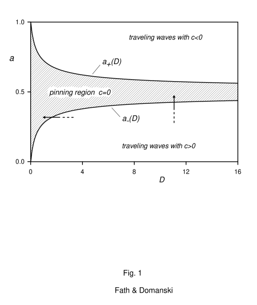
Figure 1: Phase diagram on the $a$ vs $D$ plane for an infinite chain. Pinned steady state solutions exist in the shaded region, while traveling waves exist in the unshaded ones. The pinning transition takes place along the $a=a_{+}(D)$ and the $a=a_{-}(D)$ curves, and can be initiated either by changing $D$ for $a$ fixed, or by varying $a$ with $D$ fixed (see arrows).

The values of $u_{+}$ and $u_{-}$ are plotted in Fig. 1 as a function of the diffusion constant $D$. Clearly, the obtained kink-$M$ steady state solution is only valid in the shaded region of the diagram. On the other hand, when $(D,a)$ is outside the shaded domain, the solution in Eqs. (7)–(9) is only a spurious solution. In this region of $(D,a)$ there are no steady state solutions; all initial conditions develop into travelling waves.

Even though the effect of lattice pinning is alike for the case of the Nagumo-type (continuous) reaction function, exact calculation of the pinning boundaries is not feasible. A perturbative approach in the small $a$ limit was carried out in Ref. Ern . There is also an important difference how the wavefront speed $c$ scales as, for a given $a$, the diffusion canstant approaches its critical value $D_{c}=D_{c}(a)$. Simple bifurcation theory analysisErn shows that in the continuous $F(u)$ case $c$ scales following a power law with an exponent $1/2$, i.e.,

$$c\sim(D-D_{c})^{1/2}$$ (13)

while for the piece-wise linear kinetics the singularity is logarithmic

$$c\sim-1/\ln(D-D_{c}).$$ (14)

The latter form arises essentially from the nonanalicity (jump discontinuity) of the $F(u)$ function in Eq. (3), and has been analysed in detail in Ref. Fath .

IV Induction with hysteresis

Let us know investigate the inductive situation. As the signal $S$ increases the distribution of concentration values $u_{n}(t)$ in the system becomes monotonically decreasing as a function of $n$. Even when the system is not in an equilibrium state we can define an $M$ value characterizing the actual position of the domain wall separating type-1 and type-0 cells using Eq. (6). When seeking a steady state kink at site $M$, we solve the semi-infinite set of equations defined by Eqs. (1) and (2) with $\partial u_{n}(t)/\partial t=0$. Again, the analytic solution is attainable for the piece-wise linearized kinetics. Working with the Ansatz

$$u_{n}=\left\{\begin{array}[]{ll}1+Ae^{n\kappa}+Be^{-n\kappa}&\mbox{if $n\leq M$}\\ Ce^{-n\kappa}&\mbox{if $n\geq M+1$}\end{array}\right.,$$ (15)

the unknown coefficients turn out to be

$$A = -\frac{1}{e^{\kappa}+1}e^{-M\kappa}$$ (16)

$$B = (e^{\kappa}-1)S-\frac{e^{\kappa}}{e^{\kappa}+1}e^{-M\kappa}$$ (17)

$$C = (e^{\kappa}-1)S+\frac{e^{\kappa}}{e^{\kappa}+1}(e^{M\kappa}-e^{-M\kappa})$$ (18)

with $\kappa$ again given by Eq. (8). Unlike in the translation invariant (infinite chain) case in Eq. (10), the concentration values at the kink, $u^{M}_{L}$ and $u^{M}_{R}$, are now explicite functions of the kink position $M$ and the signal strength $S$

$$u^{M}_{L}(S)=(e^{\kappa}-1)e^{-M\kappa}S+\frac{e^{\kappa}}{e^{\kappa}+1}(1-e^{-2M\kappa})$$

$$u^{M}_{R}(S)=e^{-\kappa}u^{M}_{L}.$$ (19)

In the limit $M\to\infty$ we get back the bulk results in Eq. (10).

As it was done for the infinite system, consistency of the solution must be checked at this point. When the consistency condition of Eq. (11) fails no steady state solution with the kink at site $M$ exists. As a consequence the process of differentiation cannot stop at site $M$, and the domain wall moves on.

Since the explicit expression for $u^{M}_{L}(S)$ and $u^{M}_{R}(S)$ is available in Eq. (19), for any values of $\beta,D,a$ and $S$ we can readily construct the set of possible $M$ values $\{M\}$ for which the consistency condition in Eq. (11) holds, and thus the kink-$M$ steady state exists. Although in theory every element of this set $\{M\}$ could be realized as a steady state, it is the previous history of the system (the initial conditions) and the dynamics of the reaction-diffusion process which determines which steady state (if any) gets finally realized. This is in contrast with the continuum space model description where the position of a steady-state kink is always uniquely determined by the actual model parameters.

The set of possible steady states on the $a$ vs $S$ plane for the case $\beta=1,D=2$ fixed is depicted in Fig. 2. The different domains are separated by straight lines which is an artifact stemming from the simple form of $F(u)$ in Eq. (3). Nevertheless, a qualitatively similar diagram can be obtained using the continuous Nagumo form. There are three main possibilities for a given $a$ and $S$: (i) the number of steady states is finite, (ii) any $M$ yields a valid steady state above a certain value (this is indicated by a ”+”), (iii) there are no steady state kinks at all.

In the piece-wise linear model under investigation the kink steady states, if they exist, are always stable against perturbations.Fath Thus if at a given time $t$ the actual kink position is not an element of the set of steady states $\{M\}$, differentiation or de-differentiation continues untill the domain wall reaches the first $M$ value which is already in $\{M\}$. Having reached the domain of attraction of a stable steady state the kink stabilizes at that point and the process halts untill, eventually, a further change in $S$ destabilizes the system again.

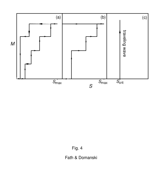
Figure 4: Schematic hysteresis diagrams for the signaling scheme $S:\;0\to S_{\rm max}\to 0$ showing the actual domain wall position $M$ as a function of the signal strength $S$. (a) all cells de-differentiate, (b) some cells remain differentiated, (c) all cells become differentiated as a travelling wave emerges.

Let us consider now an adiabatically slow process in which the inductive signal increases from zero to $S_{\rm max}$ and then decreases back to zero again. Using the above rule we can easily construct the phase diagram shown in Fig. 3 for such a process. Domains are labelled by the $M$ values of the kinks as they get realized in order. For example, the small domain $[01230]$ has a history in which $M$ increases continuously from 0 to 3, then as the signal diminishes it jumps ubruptly back to 0. Once again there are three main regions, separated by thick lines, in this phase diagram:
(i) In the upper part of the phase diagram the system gradually differentiates and then completely de-differentiates as the signal varies. The de-differentiation process can be continuous or may contain sudden jumps when the value of $a$ is closer to $u_{+}$. Note that this region corresponds more or less to the values of $a$ where in the infinite model kinks develop into travelling waves moving leftwards, i.e. towards the surface of our semi-infinite system. Due to this bias a continuous presence of the signal is needed to maintain differentiated type-1 cells in the system.
(ii) In the middle part of the phase diagram, corresponding approximatively to the pinning region of Fig. 1, the cells remain differentiated even when $S$ falls back to zero. Note that when $a$ is close to $u_{-}$ the domain wall can take a huge jump at the beginning as $S$ reaches a certain value. In this situation the maximum value of the signal $S_{\rm max}$ is important, since this is the factor which determines the range of the irreversibly differentiated domain.
(iii) Finally for small values of $a$ the differentiation process becomes self-sustaining when a critical value of the signal is exceeded. This mimics the infinite chain behaviour with a travelling wave moving rightwards. The signal only triggers the differentiation process but after that it plays no further role.
Typical examples of the three kinds of behavior are depicted in Fig. 4(a-c).

The structure of the phase diagram in Fig. 3 is rather involved, demonstrating that even a simple model like this can show an amazing complexity. When the more realistic Nagumo-type reaction function is considered the exact solvability of the problem is lost. Nevertheless, numerical simulations we carried out demonstrated that the main conclusions about the qualitative behavior of the three phases remain unchanged.

V Summary and discussion

In this paper we analysed a semi-infinite one-dimensional one-chemical reaction-diffusion system. The reaction kinetics was assumed to be bistable, giving rise to two different type of cells: type-0 (low concentration type) and type-1 (high concentration type). Starting from a homogeneous situation (all cell are type-0) the system underwent a differentiation process in response to an external inductive signal. The signal was modelled as a boundary condition in the continuum version and as an extra term in the internal cell kinetics of the first cell in the discrete space version.

Depending on the model parameters the differentiation process sweeps through the whole system, or flips a limited number of cells to type-1 up to a given position. We found that the behavior of the system differs considerably in the continuum and in the discrete space versions. In the former the position of the domain wall between the two cell types is either a well-defined function of the external signal strength, or the front of differentiation inevitably develops into a travelling wave. In the discrete case the fate of the system depends on its previous history, giving rise to hysteresis.

We analysed in detail the situation when the bistable reaction function is piece-wise linear. The model was solved analytically, and we constructed a detailed phase diagram based on the different types of behavior as a function of the model parameters. We found three mayor scenarios for the system: (i) In response to the inductive signal the solution develops into a travelling wave which differentiates the whole (semi-infinite) domain, (ii) the signal causes some spatially limited differentiation but when it diminishes all cells de-differentiate, (iii) differentiated cells get stabilized and the inhomogenious solution persists even when the signal disappears.

Although the analysis was carried out with a somewhat special reaction function, numerical simulations we have done support our expectation that the observed behavior is widely universal in discrete space models, and the qualitative chategories found remain valid in similar models with more realistic reaction functions. There are, of course, minor quantitative differences such as the type of scaling near the bifurcation points, or the actual domain wall location for a given signaling scheme.

In general we have found that adding spatial discreteness to reaction diffusion models has a tendency to improve domain wall stability between different tissues, and to make the emerging pattern less susceptible to fluctuations of the signaling mechanisms. Since robostness and stability of developmental processes and that of the adult organism is an inevitable necessity for the survival of biological species, we may wonder that the invention of cellular membranes by evolution, which made the fundamental building blocks discrete, was at least in parts motivated by such a developmental benefit, among others.

Finally we would like to mention an actual biological observation which seems to be explainable on the basis of the above model. During the retina differentiation of Drosophila it has been observed that ommatidia (the basic functional units of the retina consisted of photoreceptor and other types of cells) develop behind a slowly moving wave front, the ”morphogenetic furrow”.retina There are many genes which are only expressed behind the furrow, and thus one (or more) of them is believed to play the role of a morphogene. It was also noticedKoc-Mei that a slight shift in the environmental temperature is enough to make the wave front stop. Untill the temperature is raised back to normal again the process of differentiation does not continue. This slight artificial manipulation, although capable of empeeding the propagation of the front for hours or days, is believed to have no residual effects on further retina development.

Knowing that the propagating wavefront is extremely slow, $c\approx?m/s$, we can speculate that the developing retina is in fact tuned very close to a pinning region boundary. A change in the tissue temperature necessarily alters the actual model parameters. Although it would be very difficult to estimate on a phenomenological basis how the complex, non-linear set of biochemical reactions get modified by a temperature decrese, we can at least assume that the overall diffusivity of the chemicals get reduced. This can drive the system into the pinning region as is illustrated in Fig. fig:bulk, causing eventually a propagation failure. In this unfavorable temperature regime the domain wall, represented by the morphogenetic furrow, between undifferentiated and already differentiated cells becomes a stable steady state, and the differentiation process temporarily halts.

Valuable discussions with Paul Erdős are acknowledged. This research was supported by the Swiss National Science Foundation Grant No. 20-37642.93.

Figure 2: Steady state kink solutions on the $a$ vs $S$ plane with $D=2$. The set $\{M_{1}M_{2}\cdots\}$ denotes the possible positions of the kinks in the given region. A ”+” represents that all $M$ values are possible above the preceding value. In the shaded regimes many small phases appear.

Figure 3: Phase diagram for the signaling scheme $S:\;0\to S_{\rm max}\to 0$ on the $a$ vs $S_{\rm max}$ plane with $D=2$. The symbol $[M_{1}M_{2}\cdots]$ denotes the order of kink positions as they get realized. In the shaded regime many small phases appear.

References

- (1) On leave from the Research Institute for Solid State Physics, Budapest, Hungary.
- (2) S. F. Gilbert: Developmental Biology, 5th ed., Sinauer Associates, 1997.
- (3) J. D. Murray: Mathematical Biology, Lecture Notes in Biomathematics vol. 19, 2nd ed., Springer-Verlag, 1993.
- (4) S. A. Kauffman: The origins of order: self-organization and selection in evolution, Oxford University Press, 1993.
- (5) A. Turing, Phil. Trans. B 237, 37 (1952).
- (6) Refs for vulva formation in C elegans.
- (7) Refs for Drosophila’s retina
- (8) D. G. Aronson and H. F. Weinberger, Adv. Math. 30, 33 (1978); P. C. Fife and J. B. McLeod, Arch. Rational Mech. Anal. 65, 333 (1977).
- (9) J. P. Keener, SIAM J. Appl. Math. 47, 556 (1987); J. Theor. Biol. 148, 49 (1991); B. Zinner, SIAM J. Math. Anal. 22, 1016 (1991); J. Diff. Eqns. 96, 1 (1992); J. P. Laplante and T. Erneux, J. Phys. Chem. 96, 4931 (1992); T. Sobrino, M. Alonso, V. Perez-Munuzuri and V. Perez-Villar, Eur. J. Phys. 14, 74 (1993); P. C. Bressloff and G. Rowlands. Physica D 106, 255 (1997); J. Rinzel, Ann. NY Acad. Sci. 591, 51 (1990).
- (10) G. Fáth, Physica D 116, 176 (1998).
- (11) T. Erneux and G. Nicolis, Physica D 67, 237 (1993).
- (12) A. J. Koch and H. Meinhardt, Rev. Mod. Phys. 66, 1481 (1994).