Also at ]Jawaharlal Nehru Centre For Advanced Scientific Research, Jakkur, Bangalore, India

The Varieties of Dynamic Multiscaling in Fluid Turbulence

Abstract

We show that different ways of extracting time scales from time-dependent velocity structure functions lead to different dynamic-multiscaling exponents in fluid turbulence. These exponents are related to equal-time multiscaling exponents by different classes of bridge relations which we derive. We check this explicitly by detailed numerical simulations of the GOY shell model for fluid turbulence. Our results can be generalized to any system in which both equal-time and time-dependent structure functions show multiscaling.

The dynamic scaling of time-dependent correlation functions in the vicinity of a critical point was understood soon after the scaling of equal-time correlations hoh77 . By contrast, the development of an understanding of the dynamic mutiscaling of time-dependent velocity structure functions in homogeneous, isotropic fluid turbulence is still continuing; and studies of it lag far behind their analogs for the multiscaling of equal-time velocity structure functions fri96 . There are three major reasons for this: (1) The multiscaling of equal-time velocity structure functions in fluid turbulence is far more complex than the scaling of equal-time correlation functions in critical phenomena fri96 . (2) The dynamic scaling of Eulerian-velocity structure functions is dominated by sweeping effects that relate temporal and spatial scales linearly and thus lead to a trivial dynamic-scaling exponent $z_{\cal{E}}=1$, where the subscript $\cal{E}$ stands for Eulerian. (3) Even if this dominant temporal scaling because of sweeping effects is removed (see below), time-dependent velocity structure functions do not have simple scaling forms. As has been recognized in Ref. lvo97 , in the fluid-turbulence context, an infinity of dynamic-multiscaling exponents is required. These are related to the equal-time multiscaling exponents by bridge relations, one class of which were obtained in Ref. lvo97 . In the forced-Burgers-turbulence context a few bridge relations of another class were obtained in Refs. hay98 and  hay00 . If the bridge relations of Refs. lvo97 and hay98 ; hay00 are compared naively, then they disagree with each other. However, the crucial point about dynamic multiscaling, not enunciated clearly hitherto, though partially implicit in Refs. lvo97 ; hay98 ; hay00 , is that different ways of extracting time scales from time-dependent velocity structure functions yield different dynamic-multiscaling exponents that are related to the equal-time multiscaling exponents by different classes of bridge relations. We systematize such bridge relations by distinguishing three types of methods that can be used to extract time scales; these are based, respectively, on integral $I$, derivative $D$, and exit-time $E$ scales. We then derive the bridge relations for dynamic-multiscaling exponents for these three methods. Finally we check by an extensive numerical simulation that such bridge relations are satisfied in the GOY shell model for fluid turbulence.

To proceed further let us recall that in homogeneous, isotropic turbulence, the equal-time, order-$p$, velocity structure function ${\mathcal{S}}_{p}(\ell)\equiv\langle[\delta v_{\parallel}({\vec{x}},t,\ell)]^{p}\rangle\sim\ell^{\zeta_{p}}$, for $\eta_{d}\ll\ell\ll L$, where $\delta v_{\parallel}({\vec{x}},t,\ell)=[{\vec{v}}({\vec{x}}+{\vec{\ell}},t)-{\vec{v}}({\vec{x}},t)]\cdot({\vec{\ell}}/\ell)$, ${\vec{v}}({\vec{x}},t)$ is the fluid velocity at point ${\vec{x}}$ and time $t$, $L$ is the large spatial scale at which energy is injected into the system, $\eta_{d}$ is the small length scale at which viscous dissipation becomes significant, $\zeta_{p}$ is the order-$p$, equal-time multiscaling exponent, and the angular brackets denote an average over the statistical steady state of the turbulent fluid. The 1941 theory (K41) of Kolmogorov kol41 yields the simple scaling result $\zeta_{p}^{K41}=p/3$. However, experiments and simulations indicate multiscaling, i.e., $\zeta_{p}$ is a nonlinear, convex function of $p$; and the von-Kármán-Howarth relation fri96 yields $\zeta_{3}=1$. To study dynamic multiscaling we use the longitudinal, time-dependent, order-$p$ structure function lvo97

$${\mathcal{F}}_{p}(\ell,\{t_{1},\ldots,t_{p}\})\equiv\langle[\delta v_{\parallel}({\vec{x}},t_{1},\ell)\ldots\delta v_{\parallel}({\vec{x}},t_{p},\ell)]\rangle.$$ (1)

Clearly ${\mathcal{F}}_{p}(\ell,\{t_{1}=\ldots=t_{p}=0\})={\mathcal{S}}_{p}(\ell)$. We normally restrict ourselves to the simple case $t_{1}=t_{2}=\ldots=t_{q}\equiv t$ and $t_{q+1}=t_{q+2}=\ldots=t_{p}=0$, for notational simplicity write ${\mathcal{F}}_{p}(\ell,t)$, and suppress the $q$ dependence which should not affect dynamic-multiscaling exponents (see below). To remove the sweeping effects mentioned above, we must of course use quasi-Lagrangian lvo97 ; bel88 or Lagrangian kan99 velocities in Eq. (1), but we do not show this explicitly here for notational convenience. Given ${\mathcal{F}}_{p}(\ell,t)$, we can extract a characteristic time scale $\tau_{p}(\ell)$ in several different ways, as we describe later. The dynamic-multiscaling ansatz $\tau_{p}(\ell)\sim\ell^{z_{p}}$ can now be used to determine the order-$p$ dynamic-multiscaling exponents $z_{p}$. Furthermore, a naive extension of K41 to dynamic scaling mit03 yields $z_{p}^{K41}=\zeta_{2}^{K41}=2/3$ for all $p$.

In the multifractal model fri96 the velocity of a turbulent flow is assumed to possess a range of universal scaling exponents $h\in{\cal I}\equiv(h_{min},h_{max})$. For each $h$ in this range, there exists a set $\Sigma_{h}\subset\mathbb{R}^{3}$ of fractal dimension $D(h)$, such that $\frac{\delta v({\vec{r}},\ell)}{v_{L}}\propto(\frac{\ell}{L})^{h}$ for $\vec{r}\in{\Sigma}_{h}$ , with $v_{L}$ the velocity at the forcing scale $L$, whence

$$\frac{{\mathcal{S}}_{p}(\ell)}{v_{L}^{p}}\equiv\frac{\langle\delta v^{p}(\ell)\rangle}{v_{L}^{p}}\propto\int_{{\cal I}}d\mu(h)(\frac{\ell}{L})^{{\cal Z}(h)}\/,$$ (2)

where ${\cal Z}(h)=[ph+3-D(h)]$, the measure $d\mu(h)$ gives the weight of the fractal sets, and a saddle-point evaluation of the integral yields $\zeta_{p}=\underset{h}{\inf}[{\cal Z}(h)]$. The $ph$ term in ${\cal Z}(h)$ comes from $p$ factors of $(\ell/L)$ in Eq. (2); the $3-D(h)$ term comes from an additional factor of $(\ell/L)^{3-D(h)}$, which is the probability of being within a distance $\sim\ell$ of the set $\Sigma_{h}$ of dimension $D(h)$ that is embedded in three dimensions. Similarly for the time-dependent structure function

$$\frac{{\mathcal{F}}_{p}(\ell,t)}{v_{L}^{p}}\propto\int_{{\cal I}}d\mu(h)(\frac{\ell}{L})^{{\cal Z}(h)}{\cal G}^{p,h}(\frac{t}{\tau_{p,h}}),$$ (3)

where ${\cal G}^{p,h}(\frac{t}{\tau_{p,h}})$ has a characteristic decay time $\tau_{p,h}\sim\ell/\delta v(\ell)\sim\ell^{1-h}$, and ${\cal G}^{p,h}(0)=1$. If $\int_{0}^{\infty}t^{(M-1)}{\cal G}^{p,h}dt$ exists, we can define the order-$p$, degree-$M$, integral time scale

$${\cal T}^{I}_{p,M}(\ell)\equiv\biggl{[}\frac{1}{{\mathcal{S}}_{p}(\ell)}\int_{0}^{\infty}{\mathcal{F}}_{p}(\ell,t)t^{(M-1)}dt\biggl{]}^{(1/M)}.$$ (4)

We can now define the integral dynamic-multiscaling exponents $z^{I}_{p,M}$ via ${\cal T}^{I}_{p,M}\sim\ell^{z^{I}_{p,M}}$. By substituting the multifractal form (3) in Eq. (4), computing the time integral first, and then performing the integration over the multifractal measure by the saddle-point method, we obtain the integral bridge relations

$$z^{I}_{p,M}=1+[\zeta_{p-M}-\zeta_{p}]/M,$$ (5)

which was first obtained in Ref. lvo97 . Likewise, if $\frac{\partial^{M}}{\partial t^{M}}{\cal G}^{p,h}|_{t=0}$ exists, we can define the order-$p$, degree-$M$, derivative time scale

$${\cal T}^{D}_{p,M}\equiv\biggl{[}\frac{1}{{\mathcal{S}}_{p}(\ell)}\frac{\partial^{M}}{\partial t^{M}}{\mathcal{F}}_{p}(\ell,t)\biggl{|}_{t=0}\biggl{]}^{(-1/M)},$$ (6)

the derivative dynamic-multiscaling exponents $z^{D}_{p,M}$ via ${\cal T}^{D}_{p,M}\sim\ell^{z^{D}_{p,M}}$, and thence obtain the derivative bridge relation

$$z^{D}_{p,M}=1+[\zeta_{p}-\zeta_{p+M}]/M.$$ (7)

Such derivative bridge relations, for the special cases (a) $p=2,M=1$ and (b) $p=2,M=2$, were first obtained in the forced-Burgers-turbulence context in Refs. hay00 and hay98 , respectively foot-jh , without using quasi-Lagrangian velocities but by using other methods to suppress sweeping effects. Case (a) yields the interesting result $z^{D}_{2,1}=\zeta_{2}$, since $\zeta_{3}=1$. Both relations (5) and (7) reduce to $z_{p}^{K41}=2/3$ if we assume K41 scaling for the equal-time structure functions.

If we consider $n$ non-zero time arguments for the structure function, ${\mathcal{F}}_{p,n}(\ell,t_{1},\ldots,t_{n},\ldots,0\ldots,0)$, which we denote by ${\mathcal{F}}_{p,n}(\ell,t_{1},\ldots,t_{n})$ for notational simplicity, we can define the integral time scale, ${\cal T}^{I}_{p,M,n}(\ell)\equiv[\frac{1}{{\mathcal{S}}_{p}(\ell)}\int_{0}^{\infty}{\mathcal{F}}_{p}(\ell,t_{1},\ldots,t_{n})t_{1}^{m_{1}-1}dt_{1}\ldots t_{n}^{m_{n}-1}dt_{n}]^{1/(Mn)},$ and the derivative time scale, ${\cal T}^{D}_{p,M,n}(\ell)\equiv[\frac{1}{{\mathcal{S}}_{p}(\ell)}\frac{\partial^{m_{1}}}{\partial t_{1}^{m_{1}}}\cdots\frac{\partial^{m_{n}}}{\partial t_{n}^{m_{n}}}{\mathcal{F}}_{p}(\ell,t_{1},\ldots,t_{n})|_{t_{1}=0,\ldots,t_{n}=0}]^{-1/(Mn)}$, where $M=\sum_{i=1}^{n}m_{i}$. From these we can obtain, as above, two generalized bridge relations :

$$z^{I}_{p,M,n}=1+(\zeta_{p-nM}-\zeta_{p})/(nM);$$

$$z^{D}_{p,M,n}=1+(\zeta_{p}-\zeta_{p+nM})/(nM).$$ (8)

In the rest of this paper, we study time-dependent structure functions of the GOY shell model for fluid turbulence fri96 ; goy73 ; kad95 :

$$(\frac{d}{dt}+\nu k_{n}^{2})u_{n}=i(a_{n}u_{n+1}u_{n+2}+$$

$$\hskip 28.45274ptb_{n}u_{n-1}u_{n+1}+c_{n}u_{n-1}u_{n-2})^{\ast}+f_{n}.$$ (9)

Here the complex, scalar velocity $u_{n}\/$, for the shell $n\/$, depends on the one-dimensional, logarithmically spaced wavevectors $k_{n}=k_{0}2^{n}\/$, complex conjugation is denoted by $\ast$, and the coefficients $a_{n}=k_{n}$, $b_{n}=-\delta k_{n-1}$, and $c_{n}=-(1-\delta)k_{n-2}$, with $\delta=1/2$, are chosen to conserve the shell-model analogs of energy and helicity in the inviscid, unforced limit. By construction, the velocity in a given shell is affected directly only by velocities in nearest- and next-nearest-neighbor shells. By contrast, all Fourier modes of the velocity field interact with each other in the Navier-Stokes equation as can be seen easily by writing it in wave-vector space. Thus the GOY shell model does not have the sweeping effect by which modes (eddies) corresponding to the largest length scales affect all those at smaller length scales directly. Hence it has been suggested that the GOY shell model should be thought of as a model for quasi-Lagrangian velocities bif99 . We might anticipate therefore that GOY-model structure functions should not have the trivial dynamic scaling associated with Eulerian velocities; we show this explicitly below. We integrate the GOY model (9) by using the slaved, Adams-Bashforth scheme  dha97 ; pis93 , and $22$ shells ($1\leq n\leq 22$), with $f_{n}=0\/$ for $n\geq 2\/$ and $f_{1}=(1+i)\times 5\times 10^{-3}$(Table 1). The equal-time structure function of order-$p$ and the associated exponent is defined by $S_{p}(k_{n})=\langle|u_{n}|^{p}\rangle\sim k_{n}^{-\zeta_{p}}$. However, the static solution of Eq. (9) exhibits a 3-cycle with the shell index $n$, which is effectively filtered out kad95 if we use $\Sigma_{p}(k_{n})\equiv\langle|\Im(u_{n+2}u_{n+1}u_{n}-(1/4)u_{n-1}u_{n}u_{n+1})|^{p/3}\rangle\sim k_{n}^{-\zeta_{p}},$ to determine $\zeta_{p}$. These exponents are in close agreement with those found for homogeneous, isotropic fluid turbulence in three dimension kad95 . Data for the exponents $\zeta_{p}$ from our calculations are given in Table 2. We analyse the velocity $(u_{n}(t))$ time-series for $n=4$ to $13$, which corresponds to wave-vectors well within the inertial range. The smaller the wave-vector $k_{n}$ the slower is the evolution of $u_{n}(t)$, so it is important to use different temporal sampling rates for velocities in different shells. We use sampling rates of $50\times\delta t$ for $4\leq n\leq 8$ and $10\times\delta t$ for $9\leq n\leq 13$, respectively.

$\nu$ $\delta t$ $\lambda$ $u_{rms}$ $Re_{\lambda}$ $L_{int}$ $\tau_{L}$ $T_{tr}$ $T_{av}$ $10^{-7}$ $2\times 10^{-4}$ $0.7$ $0.35$ $2\times 10^{6}$ $6.3$ $10^{5}\delta t$ $5\times 10^{4}\delta t$ $10^{5}\tau_{L}$

Table 1: Viscosity $\nu$, the time-step $\delta t$, Taylor microscale $\lambda\equiv(\sum_{n}|u_{n}|^{2}/k_{n}/\sum_{n}k_{n}|u_{n}|^{2})^{1/2}$, the root-mean-square velocity $u_{rms}\equiv[2\sum_{n}|u_{n}|^{2}/k_{n}/(2\pi k_{1})]^{1/2}$, the Taylor-microscale Reynolds number $Re_{\lambda}\equiv\lambda u_{rms}/\nu$, the integral scale $L_{int}\equiv(\sum_{n}|u_{n}|^{2}/k_{n}^{2})/(\sum_{n}|u_{n}|^{2}/k_{n})$, and the box-size eddy turnover time $\tau_{L}\equiv L_{int}/u_{rms}$, that we use in our numerical simulation of the GOY shell model. Data from the first $T_{tr}$ time steps are discarded so that transients can die down. We then average our data for time-dependent structure functions for an averaging time $T_{av}$.

For the GOY shell model we use the normalized, order-$p$, complex, time-dependent structure function, $f_{p}(n,t)\equiv\langle[u_{n}(0)u_{n}^{*}(t)]^{p/2}\rangle/S_{p}(k_{n})$ , which has both real and imaginary parts. The representative plot of Fig. 1 shows that the imaginary part of $f_{p}(n,t)$ is negligibly small compared to its real part. Hence we work with the real part of $f_{p}(n,t)$, i.e., $F_{p}(n,t)\equiv\Re[f_{p}(n,t)]$.

Integral and derivative time scales can be defined for the shell model (9) as in Eqs. (4) and (6). We now concentrate on the integral time scale with $M=1$, $T^{I}_{p,1}(n,t_{u})\equiv\int_{0}^{t_{u}}F_{p}(n,t)dt$, the derivative time scale with $M=2$, $T^{D}_{p,2}\equiv[\frac{\partial^{2}F_{p}(n,t)}{\partial t^{2}}|_{t=0}]^{-1/2}$, and the associated dynamic-multiscaling exponents defined via $T^{I}_{p,1}(n,t_{u})\sim k_{n}^{-z^{I}_{p,1}}$ and $T^{D}_{p,2}(n)\sim k_{n}^{-z^{D}_{p,2}}$. In principle we should use $t_{u}\rightarrow\infty$ but, since it is not possible to obtain $F_{p}(n,t)$ accurately for large $t$, we select an upper cut-off $t_{u}$ such that $F_{p}(n,t_{u})=\alpha$, where, for all $n$ and $p$, we choose $\alpha=0.7$ in the results we report. We have checked that our results do not change if we use $0.3<\alpha<0.8$. The slope of a log-log plot of $T^{I}_{p,1}(n)$ versus $k_{n}$ now yields $z^{I}_{p,1}$ (Fig. 1 and Table 2). Preliminary data for $z^{I}_{p,1}$ were reported by us in Ref. mit03 .

For extracting the derivative scale $T^{D}_{p,2}$ we extend $F_{p}(n,t)$ to negative $t$ via $F_{p}(n,-t)=F_{p}(n,t)$ and use a centered, sixth-order, finite-difference scheme to find $\frac{\partial^{2}}{\partial t^{2}}F_{p}(n,t)|_{t=0}$. A log-log plot of $T^{D}_{p,2}(n)$ versus $k_{n}$ now yields the exponent $z^{D}_{p,2}$ (Fig. 1 and Table 2).

In Ref. bif99 dynamic-multiscaling exponents were extracted not from time-dependent structure functions but by using the following exit-time algorithm: We define the decorrelation time for shell $n$, at time $t_{i}$, to be $T_{i}(n)$, such that, $|u_{n}(t_{i})||u_{n}(t_{i}+T_{i})|\geq\lambda^{\pm 1}|u_{n}(t_{i})|^{2}$, with $0<\lambda<1$. The exit-time scale of order-$p$ and degree-$M$ for the shell $k_{n}$ is

$$T^{E}_{p,M}\equiv\underset{N\rightarrow\infty}{\lim}\biggl{[}\frac{\frac{1}{N}\sum_{i=1}^{N}T_{i}^{M}|u_{n}(t_{i})|^{p}}{\frac{1}{N}\sum_{i=1}^{N}|u_{n}(t_{i})|^{p}}\biggl{]}\sim k_{n}^{-z^{E}_{p,M}},$$ (10)

where the last proportionality follows from the dynamic-multiscaling ansatz. In practice we cannot of course take the limit $N\rightarrow\infty$; in a typical run of length $T_{av}$ (Table 1) $N\simeq 10^{9}$. By suitably adapting the multifractal formalism used above, we get the exit-time bridge relation $z^{E}_{p,M}=1+[\zeta_{p-M}-\zeta_{p}]/M$, obtained in Ref. bif99 only for $M=1$. Dynamic-multiscaling exponents obtained via this exit-time algorithm are shown for $M=1$ and $M=-2$ in Table 2. The exit-time bridge relations for $M>0$ are the analogs of the integral-time bridge relation (5) and those for $M<0$ are the analogs of the derivative-time bridge relation (7). We have checked that our results do not depend on $\lambda$ for $0.3<\lambda<0.8$.

Our numerical results for the equal-time exponents $\zeta_{p}$ (Column 2), the integral-time exponents $z^{I}_{p,1}$ (Columns 3 and 4), the derivative-time exponents $z^{D}_{p,2}$ (Columns 6 and 7), and the exit-time exponents $z^{E}_{p,1}$ and $z^{E}_{p,-2}$ (Columns 5 and 8, respectively) for $1\leq p\leq 6$ are given in Table 2. The agreement of the exponents in Columns 3 and 4 shows that the bridge relation (5) is satisfied (within error bars). Likewise, a comparison of Columns 6 and 7 shows that the bridge relation (7) is satisfied. By comparing Columns 4 and 5 we see that the integral-time exponent $z^{I}_{p,1}$ is the same as the exit-time exponent $z^{E}_{p,1}$; similarly, Columns 7 and 8 show that the derivative-time exponent $z^{D}_{p,2}$ is the same as the exit-time exponent $z^{E}_{p,-2}$. The relation $z^{D}_{2,1}=\zeta_{2}$ mentioned above hay00 is not meaningful in the GOY model since $\partial F_{p}(n,t)/\partial t|_{t=0}$ vanishes, at least at the level of accuracy of our numerical study.

We have obtained $50$ different values of each of the dynamic-multiscaling exponents from $50$ different initial conditions. For each of these initial conditions time-averaging is done over a time $T_{av}$(Table 1) which is larger than the averaging time of Ref. bif99 by a factor of about $10^{4}$. The means of these $50$ values for each of the dynamic-multiscaling exponents are shown in Table 2; and the standard deviation yields the error. This averaging is another way of removing the effects of the 3-cycle mentioned above.

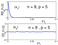
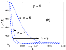
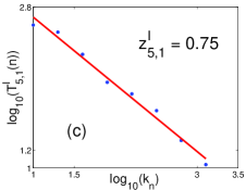
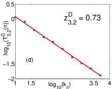
Figure 1: Plots of real (${\text{a}_{1}}$) and imaginary (${\text{a}_{2}}$) parts of the time-dependent structure function $f_{p}(n,t)$ for the GOY shell model for shell number $n=9$ and order $p=5$ versus time $t/\tau_{L}$, where $\tau_{L}$ is the box-size eddy turnover time (Table 1). Note that $\Im[f_{p}(n,t)]$ is negligibly small compared to $F_{p}(n,t)=\Re[f_{p}(n,t)]$. (b) $F_{p}(n,t)$ versus $t/\tau_{L}$ for $p=5$ and $n=5,7,$ and $9$. Representative log-log plots (base 10) of the integral (c) and derivative (d) time scales $T^{I}_{5,1}(n)$ and $T^{D}_{3,2}(n)$ versus $k_{n}$; the slopes of the linear least-square fits in (c) and (d) yield the dynamic exponents $z^{I}_{5,1}$ and $z^{D}_{3,2}$, respectively.

order$(p)$ $\zeta_{p}$ $z_{p,1}^{I}$[Eq.(5)] $z_{p,1}^{I}$ $z^{E}_{p,1}$ $z_{p,2}^{D}[Eq.(\ref{zdpm})]$ $z_{p,2}^{D}$ $z^{E}_{p,-2}$ 1 0.3777 $\pm$ 0.0001 0.6221 $\pm$ 0.0001 0.60 $\pm$ 0.02 0.603 $\pm$ 0.007 0.6820 $\pm$ 0.0001 0.70 $\pm$ 0.02 0.677 $\pm$0.001 2 0.7091 $\pm$ 0.0001 0.6686 $\pm$ 0.0002 0.67 $\pm$ 0.02 0.661$\pm$ 0.007 0.7081 $\pm$ 0.0002 0.71 $\pm$ 0.01 0.719 $\pm$0.004 3 1.0059 $\pm$ 0.0001 0.7030 $\pm$ 0.0002 0.701 $\pm$ 0.009 0.708 $\pm$ 0.001 0.7310 $\pm$ 0.0002 0.73 $\pm$ 0.01 0.739 $\pm$0.006 4 1.2762 $\pm$ 0.0002 0.7298 $\pm$ 0.0003 0.727 $\pm$ 0.007 0.74$\pm$0.01 0.7509 $\pm$ 0.0003 0.744 $\pm$ 0.009 0.758 $\pm$0.006 5 1.5254 $\pm$ 0.0005 0.7511 $\pm$ 0.0007 0.759 $\pm$ 0.009 0.77$\pm$ 0.01 0.7684 $\pm$ 0.0007 0.756 $\pm$ 0.009 0.778 $\pm$0.003 6 1.757 $\pm$ 0.001 0.768 $\pm$ 0.002 0.77 $\pm$ 0.01 0.79$\pm$ 0.01 0.7836 $\pm$ 0.002 0.764 $\pm$ 0.009 0.797 $\pm$0.0008

Table 2: Order$-p\/$ (Column 1) multiscaling exponents for $1\leq p\leq 6$ from our simulations of the GOY model: equal-time exponents $\zeta_{p}$ (Column 2), integral-scale dynamic-multiscaling exponent $z^{I}_{p,1}\/$ of degree-$1$ (Column 3) from the bridge relation (5) and the values of $\zeta_{p}$ in Column 1, $z^{I}_{p,1}$ from our calculation using time-dependent structure functions (Column 4), the exit-time exponents of order $1$ $z^{E}_{p,1}$ (Column 5), the derivative-time exponents $z^{D}_{p,2}$ (Column 6) from the bridge relation (7) and the values of $\zeta_{p}$ in Column 1, $z^{D}_{p,2}$ from our calculation using time-dependent structure function (Column 7) and the exit-time exponent of order $-2$, $z^{E}_{p,-2}$ (Column 8). The error estimates are obtained as described in the text.

We have shown systematically how different ways of extracting time scales from time-dependent velocity structure functions or time series can lead to different sets of dynamic-multiscaling exponents, which are related in turn to the equal-time multiscaling exponents $\zeta_{p}$ by different classes of bridge relations. Our extensive numerical study of the GOY shell model for fluid turbulence verifies explicitly that such bridge relations hold. Experimental studies of Lagrangian quantities in turbulence have been increasing over the past few years lag . We hope our work will stimulate studies of dynamic multiscaling in such experiments. Furthermore, the sorts of bridge relations we have discussed here must also hold in other problems with multiscaling of equal-time and time-dependent structure functions or correlation functions. Passive-scalar and magnetohydrodynamic turbulence are two obvious examples which we will report on elsewhere mit . Numerical studies of time-dependent, quasi-Lagrangian-velocity structure functions in the Navier-Stokes equation, already under way, will also be discussed elsewhere.

We thank A. Celani, S.K. Dhar, U. Frisch, S. Ramaswamy, A. Sain, and especially C. Jayaprakash for discussions. This work was supported by the Indo-French Centre for the Promotion of Advanced Research (IFCPAR Project No. 2404-2). D.M. thanks the Council of Scientific and Industrial Research, India for support.

References

- (1) P. C. Hohenberg and B. I. Halperin, Rev. Mod. Phys. 49 435 (1977) and references therein.
- (2) U. Frisch, Turbulence: The Legacy of A.N. Kolmogorov (Cambridge University Press, Cambridge, 1996).
- (3) V.S. L’vov, E. Podivilov, and I. Procaccia, Phys. Rev. E 55 7030 (1997).
- (4) F. Hayot and C. Jayaprakash, Phys. Rev. E 57 R4867 (1998).
- (5) F. Hayot and C. Jayaprakash, Int. J. Mod. Phys. B, 14, 1781 (2000).
- (6) A.N. Kolmogorov, Dokl. Acad. Nauk USSR 30 9 (1941).
- (7) V.I. Belinicher and V.S. L’vov, Sov. Phys. JETP 66 303 (1987).
- (8) Y. Kaneda, T. Ishihara, and K. Gotoh, Phys. Fluids 11 2154 (1999).
- (9) D. Mitra and R. Pandit, Physica A 318 179 (2003).
- (10) In Ref. hay98 case (b) appears as a sub-dominant contribution to the dominant sweeping contribution.
- (11) E.B. Gledzer, Sov. Phys. Dokl. 18 216 (1973); K. Ohkitani and M. Yamada, Prog. Theor. Phys. 81 329 (1989).
- (12) L.P. Kadanoff, D. Lohse, J. Wang, and R. Benzi, Phys. Fluids 7 617 (1995).
- (13) L. Biferale, G. Bofetta, A. Celani, and F. Toschi, Physica D 127 187 (1999).
- (14) S.K. Dhar, A. Sain, and R. Pandit, Phys. Rev. Lett. 78 2964 (1997).
- (15) D. Pisarenko, L. Biferale, D. Courvoisier, U. Frisch, and M. Vergassola, Phys. Fluids A 5 2533 (1993).
- (16) See, e.g., S. Ott and J. Mann, J. Fluid Mech. 422 207 (2000); A. La Porta, G.A. Voth, A.M. Crawford, J. Alexander, and E. Bodenschatz, Nature(London) 409 (2002); N. Mordant, P. Metz, O. Michel, and J.-F. Pinton, Phys. Rev. Lett. 87 214501 (2001).
- (17) D. Mitra and R. Pandit, to be published.