Onset and universality of drag reduction in the turbulent Kolmogorov flow

Abstract

We investigate the phenomenon of drag reduction in a viscoelastic fluid model of dilute polymer solutions. By means of direct numerical simulations of the three-dimensional turbulent Kolmogorov flow we show that drag reduction takes place above a critical Reynolds number $Re_{c}$. An explicit expression for the dependence of $Re_{c}$ on polymer elasticity and diffusivity is derived. The values of the drag coefficient obtained for different fluid parameters collapse onto a universal curve when plotted as a function of the rescaled Reynolds number $Re/Re_{c}$. The analysis of the momentum budget allows to gain some insight on the physics of drag reduction, and suggests the existence of a maximum drag reduction asymptote for this flow.

When a viscous fluid is kept in motion by some external driving, a mean flow is established: the ratio between the work made by the force and the kinetic energy carried by the mean flow is called the drag coefficient, or friction factor. This dimensionless number measures the power that has to be supplied to the fluid to maintain a given throughput. When the flow is laminar, the drag coefficient is inversely proportional to the Reynolds number. Upon increasing the intensity of the applied force the flow eventually becomes turbulent, and the drag coefficient becomes approximately independent of the Reynolds number R1883 , therefore substantially larger than in the viscous case.

In 1949 the British chemist Toms reported that the turbulent drag could be reduced by up to 80% through the addition of minute amounts (few tenths of p.p.m. in weight) of long-chain soluble polymers to water. This observation triggered an enormous experimental activity to characterize this phenomenon (see, e.g., L69 ; V75 ; MC92 ; NH95 ; SW00 ). In spite of these efforts, no fully satisfactory theory of drag reduction is available yet. However, a recent breakthrough has been the observation of drag reduction in numerical simulations of the turbulent channel flow of viscoelastic fluids SBH97 . Most of the features of experimental flows of dilute polymer solutions are successfully reproduced by these models, even at the quantitative level PBNHVH03 . Despite these advances, the understanding of drag reduction in the experimentally relevant geometry of pipe or channel flow is still hindered by the complexity of these flows already at the Newtonian level, i.e. in the absence of polymers DCLPP03 . This consideration motivated us to investigate simpler geometries in the hope that this may shed some light on the basic physical mechanisms of drag reduction (see, e.g., Ref. DCBP02 ).

In this Letter we present the results of an extensive numerical investigation of the viscoelastic turbulent Kolmogorov flow. This system has several analogies with the turbulent channel flow, while its main distinctive trait is the absence of material boundaries. Notwithstanding this major difference we will show that drag reduction takes place in the Kolmogorov flow as well. Furthermore, we observe striking quantitative similarities with experimental results in wall-bounded flows: this points to the conclusion that the basic physical mechanisms of drag reduction be substantially independent of the detailed structure of the flow.

To describe the dynamics of a dilute polymer solution we adopt the linear viscoelastic model (Oldroyd-B) BCAH87

$$\partial_{t}{\bm{u}}+({\bm{u}}\cdot{\bm{\nabla}}){\bm{u}}=-{\bm{\nabla}p}+\nu_{0}{\Delta}{\bm{u}}+\frac{2\eta\,\nu_{0}}{\tau}{\bm{\nabla}}\cdot{\bm{\sigma}}+{\bm{F}},$$ (1)

$$\partial_{t}{\bm{\sigma}}+({\bm{u}}\cdot{\bm{\nabla}}){\bm{\sigma}}\!=\!({\bm{\nabla}\bm{u}})^{T}\!\cdot{\bm{\sigma}}+{\bm{\sigma}}\!\cdot({\bm{\nabla}\bm{u}})-2\frac{{\bm{\sigma}}-{\bm{1}}}{\tau}+\kappa\Delta{\bm{\sigma}}.$$ (2)

The velocity field ${\bm{u}}$ is incompressible, the symmetric matrix ${\bm{\sigma}}$ is the conformation tensor of polymer molecules, and its trace $\textrm{tr}{\bm{\sigma}}$ is a measure of their elongation. The parameter $\tau$ is the (slowest) polymer relaxation time. The matrix of velocity gradients is defined as $({\bm{\nabla}\bm{u}})_{ij}=\partial_{i}u_{j}$ and ${\bm{1}}$ is the unit tensor. The solvent viscosity is denoted by $\nu_{0}$ and $\eta$ is the zero-shear contribution of polymers to the total solution viscosity $\nu=\nu_{0}(1+\eta)$. The parameter $\eta$ is proportional to the polymer concentration. The diffusive term $\kappa\Delta{\bm{\sigma}}$ is added to prevent numerical instabilities SB95 . The constant forcing ${\bm{F}}=(F\cos(z/L),0,0)$ maintains the system in a statistically stationary state characterized by a mean flow $\langle{\bm{u}}\rangle$. Due to the symmetries of ${\bm{F}}$, the only nonzero component of the mean velocity is $\langle u_{x}\rangle$: it depends on the shear coordinate $z$ alone, vanishes at $z=\pm(\pi/2)L$, and is even under reflections $z\to-z$. Its value at $z=0$, $\langle u_{x}\rangle_{z=0}$, will be denoted by $U$. Finally, we establish a short glossary between the Kolmogorov flow and the channel flow: $F$ plays the role of the pressure gradient, $\pi L$ is analogous to the channel height, and $U$ is equivalent to the centerline velocity.

In this framework, we have performed a series of numerical integrations of eqs. (1) and (2) for a set of values of forcing intensity $F$, at fixed $\nu$, both for the Newtonian and the viscoelastic case. Comparing results at a given $F$ is equivalent to keeping an imposed pressure gradient – therefore a fixed wall-shear stress – in channel flow experiments (see, e.g. Ref. LT88 ). We have measured the mean profiles of several relevant observables, including the average velocity $\langle u_{x}\rangle$, the turbulent shear stress (Reynolds stress) $\langle u_{x}u_{z}\rangle$, and the mean polymer stress $2\nu_{0}\eta\tau^{-1}\langle\sigma_{xz}\rangle$. The mean flow is accurately described by the sinusoidal profile $\langle u_{x}\rangle=U\cos(z/L)$, both in the Newtonian and in the viscoelastic flow profiles .

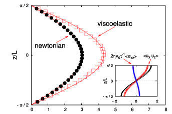
Figure 1: Mean velocity profiles for a Newtonian ($\eta=0$) and a viscoelastic simulation ($\eta=0.3$, $El=0.019$) at given forcing amplitude $F=1.5$. The measured profiles are undistinguishable from $\langle u_{x}\rangle=U\cos(z/L)$ (full lines) in both cases. The effect of elasticity is to increase the peak value $U$ with respect to the Newtonian case: in the present case this corresponds to a reduction of the drag coefficient, defined in eq. (3), of about $40\%$. In the inset, the profiles of the Reynolds stress $\langle u_{x}u_{z}\rangle=S\sin(z/L)$ and the mean polymer stress $2\nu_{0}\eta\tau^{-1}\langle\sigma_{xz}\rangle=-T\sin(z/L)$. In this case the Reynolds stress is reduced upon polymer addition to approximately $70\%$ of its Newtonian value, consistently with experimental results at comparable drag reduction WWL87 . The ”missing” turbulent shear stress is compensated by the contribution of the polymer stress: the sum of $S$ and $T$ is equal to $F$ in both the Newtonian and viscoelastic case. Data result from the numerical integration of eqs. (1) and (2) in a periodic cube of side $2\pi$ by means of a fully dealiased pseudospectral code with $64^{3}$ collocation points. The mean flow lengthscale is $L=1$ and the viscosity is $\nu=0.015625$. Starting from an initial configuration with a small amount of energy on the smallest modes, after the system evolved into a statistically stationary state, time averages over 100 to 1000 eddy-turnover times have been performed to obtain the mean velocity profiles.

However, as shown in Fig. 1, in the latter case the centerline velocity $U$ is definitely larger: this is the hallmark of drag reduction. It has to be remarked that – at variance with wall-bounded flows where drag reduction is always accompanied by a structural change in the profile (see e.g. Ref. V75 ) – in the Kolmogorov flow the increase in throughput takes place just by means of an overall rescaling of the mean velocity. This is due to the different boundary conditions: in channel flows, the profile in the viscous sublayer is left unchanged upon polymer addition while the bulk flow increases substantially. This requires a reshaping of the mean profile, that takes actually place through the increase of the extent of the buffer region (see e.g. Ref. LT88 ). In the Kolmogorov flow there is no constraint on velocity profiles, and drag reduction does not necessarily entail their structural change.

To quantify the effect of viscoelasticity on the mean flow, we have defined the drag coefficient as

$$f=\frac{FL}{U^{2}}\;,$$ (3)

and measured its dependence on the Reynolds number $Re=UL/\nu$ Rey-num . For $Re<\sqrt{2}$ the flow is laminar with mean velocity $U=FL^{2}/\nu$, giving a drag coefficient $f=Re^{-1}$. At $Re\gtrsim 50$ the system is already in a fully developed turbulent state.

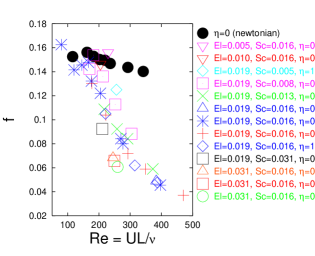
Figure 2: The drag coefficient for different viscoelastic fluid parameters. Data have been collected from numerical simulations at different forcing amplitudes $F$ and viscoelastic parameters $\eta$, $\tau$, $\kappa$. The statistical error in the determination of $f$ and $Re$ is of the order of the symbols’ size.

For a Newtonian fluid, numerical data show that the drag coefficient is approximately independent of $Re$ (see Fig. 2). This behaviour agrees with the following classical Kolmogorov argument: since the average energy input $\epsilon=FU/2$ scales as $\epsilon=\frac{\beta}{2}\,U^{3}/L$ in fully developed turbulence, eq. (3) yields a constant drag coefficient $f=\beta$. The Newtonian momentum budget gives $F_{x}=\partial_{z}\langle u_{x}u_{z}\rangle$ (the viscous contribution being negligible) and therefore a Reynolds stress $\langle u_{x}u_{z}\rangle=S\sin(z/L)$ with $S=\beta U^{2}$. For the turbulent Kolmogorov flow, $\beta\simeq 0.15$.

When polymers are added $f$ may be reduced with respect to its Newtonian value, depending on the polymer elasticity $El=\nu\tau/L^{2}$, the Schmidt number $Sc=\nu/\kappa$, and the concentration $\eta$, as shown in Fig. 2. For the highest Reynolds number we can attain in our simulations the friction factor is reduced by 75%. Drag reduction is accompanied by changes in the velocity field similar to those occurring in channel flow experiments and simulations: the level of transverse fluctuations $\langle u_{z}^{2}\rangle$ is reduced while longitudinal fluctuations $\langle(u_{x}-\langle u_{x}\rangle)^{2}\rangle$ increase and high streamwise velocity streaks are observed (see Fig. 3). Incidentally, we notice that drag reduction is observed at Reynolds numbers definitely smaller than the typical experimental values: this is possible thanks to the relatively high value of elasticity utilized in our simulations. Comparable parameters have been used in numerical simulations of the channel flow as well (see, e.g. Ref. SBH97 ), and produced a similar effect on the threshold for drag reduction.

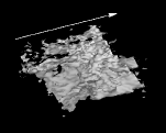
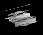
Figure 3: Snapshots of the isosurfaces $u_{x}(x,y,z)=U$ for a Newtonian (left) and a viscoelastic simulation (right, $El=0.019$, $Sc=0.016$, $\eta=0.5$). The Reynolds number is $Re\approx 350$. The arrows show the direction of the mean flow. Small-scale turbulent fluctuations, responsible for kinetic energy dissipation, are suppressed in the viscoelastic case. A high-speed streak in the form a streamwise oriented tube is visible in the viscoelastic case (right).

From the inspection of Fig. 2 we notice some systematic trend: at moderate Reynolds numbers ($Re\lesssim 200$) viscoelastic effects do not alter substantially the value of the drag coefficient; at larger $Re$ polymers with a higher elasticity are more effective as drag-reducing agents; conversely, polymers with higher diffusivity are less effective. To understand the variation of the drag coefficient with fluid parameters, we sought a dependence of the form $f=\varphi(Re/Re_{c})$ where $Re_{c}(El,Sc,\eta)$ is the critical Reynolds number for the onset of drag reduction. To obtain an explicit expression for $Re_{c}$ we need to extend the argument given in Ref. BFL01 to the case of finite polymer diffusivity. The reasoning goes as follows: for polymers to be substantially elongated, stretching must prevail over elastic relaxation and diffusivity timecr ; at the onset, the terms appearing in eq. (2) must then satisfy $(\nabla u)_{c}\sim 2/\tau+\kappa/L^{2}$; since the transition is incipient we can estimate the typical velocity gradient as $(\epsilon_{c}/\nu)^{1/2}$, and utilizing the expression $\epsilon_{c}\propto U_{c}^{3}/L$ we finally obtain

$$Re_{c}\propto\left(\frac{2}{El}+\frac{1}{Sc}\right)^{2/3}\;.$$ (4)

For vanishing diffusivity we recover the result of Ref. BFL01 . Extracting the explicit dependence on polymer concentration, we have $Re_{c}\propto(1+\eta)^{-2/3}$, which is compatible with the weak dependence on concentration found in experiments V75 .

In Fig. 4 we present the same data as in Fig. 2, now plotted against the rescaled Reynolds number $Re/Re_{c}$. The good quality of the collapse supports the validity of the relation $f=\varphi(Re/Re_{c})$. The function $\varphi$ is universal with respect to the choice of fluid parameters. Its shape will be derived in the following, with the aid of simple assumptions, starting from the equation for momentum conservation (see Ref. LPPT03 for a similar approach to wall-bounded flows).

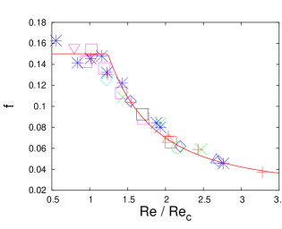
Figure 4: The drag coefficient plotted as a function of the rescaled Reynolds number $Re/Re_{c}$. Symbols as in fig. 2. The full line is eq. (5) with $\beta=0.15$, $\gamma=0.2$ and $\delta=0.02$.

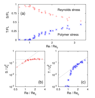
Figure 5: $(a)$: Peak values of the Reynolds stress $\langle u_{x}u_{z}\rangle=S\sin(z/L)$, and of the polymer stress $2\eta\nu_{0}\tau^{-1}\langle\sigma_{xz}\rangle=-T\sin(z/L)$, nondimensionalized by the total stress $FL$. The sum $(S+T)/(FL)$ nearly equals unity for each couple of datapoints, confirming that the viscous (solvent) stress $\nu_{0}U/L^{2}$ is negligible at the present Reynolds numbers. $(b)$ The Reynolds stress $S$ and $(c)$ the polymer stress $T$ nondimensionalized by the squared critical velocity $U_{c}^{2}$: The full lines are: $S/U_{c}^{2}=\gamma$ (left, horizontal), $S/U_{c}^{2}=\beta(Re/Re_{c})^{2}$ (left, oblique), $T/U_{c}^{2}=\delta(Re/Re_{c})^{2}$ (right). The numerical parameters are $\beta=0.15$, $\gamma=0.2$ and $\delta=0.02$.

Upon time averaging, eq. (1) reduces to $F_{x}=-\nu_{0}\partial_{z}^{2}\langle{u_{x}}\rangle+\partial_{z}(\langle{u_{x}u_{z}}\rangle-2\nu_{0}\eta\,\langle{\sigma_{xz}}\rangle/\tau)$. Utilizing the numerical observation that the Reynolds stress ${\cal S}=\langle{u_{x}u_{z}}\rangle=S\sin(z/L)$ and the polymer stress ${\cal T}=2\nu_{0}\eta\langle{\sigma_{xz}}\rangle/\tau=-T\sin(z/L)$, we obtain the momentum budget $F=\nu_{0}U/L^{2}+S/L+T/L$. The contribution $\nu_{0}U/L^{2}$ is relevant only in the laminar regime, and can therefore be neglected. The dependence of the stresses on the rescaled Reynolds number is presented in Fig. 5. Below the threshold the polymer stress is vanishingly small whereas the Reynolds stress is $S\simeq\beta U^{2}\simeq FL$ in agreement with the observation of a $Re$-independent drag coefficient. Above $Re_{c}$, the polymer stress makes a significant contribution to the momentum budget. At the largest $Re$ we can attain, the elastic stress reaches almost 50% of the total stress, not far from experimental results PNVH01 . Rescaling the stresses with the critical velocity squared shows that above the onset $S$ tends to a constant value $\gamma U_{c}^{2}$ (see Fig. 5(b)), and the polymer stress follows the law $T=\delta U^{2}$ (Fig. 5(c)). The physical interpretation of these observations is that above the onset of drag reduction an increasing fraction of the momentum injected by the external force is sequestered by polymers, which are however less effective in absorbing it than transverse velocity fluctuations ($\delta<\beta$). This results in an enhancement of the mean flow with respect to the Newtonian case, i.e. drag-reduction. Inserting the empirical expressions for $S$ and $T$, the momentum budget above the onset reads $F=\gamma U_{c}^{2}/L+\delta U^{2}/L$, and the resulting drag coefficient is

$$f=\left\{\begin{array}[]{lcc}\beta&\mbox{for}&Re\lesssim Re_{c}\,,\\ \displaystyle{\gamma\left(\frac{Re_{c}}{Re}\right)^{2}+\delta}&\mbox{for}&Re\gtrsim Re_{c}\;.\end{array}\right.$$ (5)

This expression is compared with numerical results in Fig. 4, where the values of the parameters $\gamma$ and $\delta$ have been obtained from the data shown in Fig. 5. The agreement is excellent, except possibly for $Re\approx Re_{c}$, where eq. (5) predicts an abrupt transition: from Fig. 5 this rather appears to be a smooth crossover, whose actual shape cannot be extracted by means of simple arguments. The actual values of $\beta$, $\gamma$ and $\delta$ are not of utmost importance since they are likely to depend on the details of the driving force, and therefore on the shape of the velocity profile. What is crucial to drag reduction is that $\delta<\beta$, or – in plain words – that momentum is transferred with greater ease to velocity fluctuations than to elastic ones. Understanding the reasons for this difference would disclose the basic physical mechanisms of drag reduction.

Remarkably, eq. (5) predicts a maximum drag reduction asymptote (see, e.g., Refs. V75 ; SW00 ). Indeed, by increasing the concentration, drag cannot be reduced below the asymptote $f=\delta$, independently of polymer elasticity and diffusivity. In this ultimate regime momentum transfer would take place only through polymer stresses. However, the present data do not cover a sufficient span of values of $Re$ to allow us to confirm or reject this prediction. Numerical simulations at higher resolution should allow to settle this issue.

We thank M. Chertkov, B. Eckhardt, V. Steinberg, and M. Vergassola for valuable discussions. We acknowledge the support of EU under the contract HPRN-CT-2002-00300 and of MIUR-Cofin 2001023848. Numerical simulations have been performed at CINECA (INFM parallel computing initiative).

References

- (1) O. Reynolds, Phil. Trans. R. Soc. 174, 935 (1883).
- (2) J. Lumley, Annu. Rev. Fluid Mech. 1, 367 (1969).
- (3) P. S. Virk, AIChE Journal 21, 625 (1975).
- (4) W. D. D. Mc Comb, The physics of fluid turbulence, Oxford University Press (1992).
- (5) R. H. Nadolink and W. W. Haigh, ASME Appl. Mech. Rev. 48, 351 (1995).
- (6) K. R. Sreenivasan and C. M. White, J. Fluid Mech. 409, 149 (2000).
- (7) R. Sureshkumar et al., Phys. Fluids 9, 743 (1997).
- (8) P. K. Ptasinski et al., J. Fluid Mech. 490, 251 (2003).
- (9) E. De Angelis et al., Phys. Rev. E 67, 056312 (2003).
- (10) E. De Angelis et al., http://arxiv.org/nlin.CD/0208016
- (11) R. B. Bird et al., Dynamics of polymeric fluids Vol.2, Wiley, New York (1987).
- (12) R. Sureshkumar and A. N. Beris, J. Non-Newtonian Fluid Mech. 60, 53 (1995).
- (13) T. S. Luchik, and W. G. Tiederman, J. Fluid Mech. 190, 241 (1988).
- (14) W. W. Willmarth et al., Phys. Fluids 30, 933 (1987).
- (15) Sinusoidal mean profiles were first observed in Newtonian () turbulence by V. Borue, and S. A. Orszag, J. Fluid Mech. 306, 293 (1996). See also the related work by J. V. Shebalin, and S. L. Woodruff, Phys. Fluids 9, 164 (1997).
- (16) It is natural to use the Reynolds number based on solution viscosity: indeed, for the non-shear-thinning fluid described by eqs. (1) and (2), coincides with the (kinematic) wall viscosity (see, e.g., Refs. SBH97 ; PBNHVH03 ). It is also possible to define the equivalent of the friction Reynolds number , often used in experiments: here, . In the Newtonian case .
- (17) E. Balkovsky et al., Phys. Rev. E 64, 056301 (2001).
- (18) This argument is just a revised version of the Lumley’s “time criterion” (see Ref. L69 ).
- (19) V. S. L’vov et al., http://arxiv.org/nlin.CD/0307034.
- (20) P. K. Ptasinski et al., Flow, Turbulence and Combustion 66, 159 (2001).