Geometric features of the mixing of passive scalars at high Schmidt numbers

Abstract

The mixing of passive scalars of decreasing diffusivity, advected in each case by the same three-dimensional Navier-Stokes turbulence, is studied. The mixing becomes more isotropic with decreasing diffusivity. The local flow in the vicinity of steepest negative and positive scalar gradients are in general different, and its behavior is studied for various values of the scalar diffusivity. Mixing approaches monofractal properties with diminishing diffusivity. We consider these results in the context of possible singularities of scalar dissipation.

PACS: 47.27.Eq, 47.53.+n, 47.27.Gs

Turbulent mixing of dyes or macromolecular substances can be understood by analyzing how these scalar substances are advected and diffused in a fluid medium. For small concentrations, the admixture, or scalar, is passive, or has no dynamic feedback on the flow—which is therefore determined independent of the scalar. Often, the scalar diffusivity is small compared with the viscosity of the fluid, so that their ratio, the so-called Schmidt number, $Sc=\nu/\kappa$, is large. Our interest here lies in the advection and diffusion of passive scalars for large values of $Sc$. In particular, we wish to understand the recent result from numerical simulations that turbulent mixing becomes more isotropic when $Sc$ is increased [1, 2]. This approach to isotropic state is evident from the fact that deviations from it, as quantified by odd moments of the scalar derivative along a mean scalar gradient, $\partial_{\parallel}\theta$, decrease as $Sc$ increases from 1 to 64 for a fixed Reynolds number of the flow [1].

We illustrate the issue on hand in Fig. 1, momentarily leaving aside the details of how the data were obtained. The figure shows the probability density function (PDF) of $\partial_{\parallel}\theta$ for four different values of $Sc$ keeping the Reynolds number fixed. It is clear from the figure that the distribution is quite asymmetric for $Sc=1$ but approaches symmetry as $Sc$ increases. This can be seen more quantitatively in the insets. The left inset shows the quantity $\pi(z)=[p(z)-p(-z)]/[p(z)+p(-z)]$, where $z=\partial_{\parallel}\theta/\langle(\partial_{\parallel}\theta)^{2}\rangle^{1/2}$ is the normalized scalar gradient component: smaller values of this quantity indicate smaller asymmetries. The right inset shows that a global measure of asymmetry $A$, defined by

$$A=\int_{-\infty}^{\infty}\,z^{3}p(z)\mbox{d}z/\int_{-\infty}^{\infty}\,|z|^{3}p(z)\mbox{d}z\,,$$ (1)

also decreases with increasing $Sc$. It is easily shown [3] that the asymmetry in the PDF of the scalar gradient is a measure of the anisotropy of the small-scale scalar (or mixing), so its reduction with $Sc$ is to be regarded as a direct indication that mixing becomes isotropic.

The reason for the asymmetry of the PDF for $Sc=O(1)$ has long been known to be the presence of ramp-cliff structures in the signature of the scalar field [4] whenever there is a mean gradient in the scalar alone or in both scalar and velocity. This conclusion has been reinforced by recent numerical studies [5, 6, 7]. For the present orientation of mean gradients, the exponential tail on the right of Fig. 1 arises directly from cliffs in the scalar signatures, the cliffs being related to the fronts of the scalar gradient distribution in three-dimensional space.

Analytical approaches to understanding the features shown in Fig. 1 are difficult. Significant progress has been made for the so-called Kraichnan model of passive scalars [8] in which the advecting velocity field is assumed to be Gaussian and to vary infinitely rapidly in time; for a review see [9]. For two-dimensional and isotropically forced high-$Sc$ turbulence it was possible to calculate the PDF of the scalar dissipation rate and thus predict the scaling in the tails of the PDF of scalar gradient fields [10]. This Lagrangian approach was based on a sufficient separation of pumping and diffusion time scales which is established at large $Sc$. However, even for the synthetic Kraichnan velocity field, a systematic study of anisotropy with $Sc$ has not been made (though some beginnings have occurred with respect to the $Sc$-dependence in Refs. [11]). Another approach [12], which follows Batchelor’s original model [13] of quasistatic straining motion, provides upper bounds for scalar derivative moments as functions of $Sc$. However, the problem still contains numerous open questions. For instance, it is unclear as to what changes occur in and around the ramp-cliff structures as $Sc\rightarrow\infty$. This Letter quantifies some of these changes via numerical simulation of turbulent mixing for a range of Schmidt numbers. We will particularly consider level sets of the steep gradients and relate them to the local structure of the advecting flow. The multifractal approach is known to sample efficiently the “singular” structures at small scales [14, 15, 16]. Therefore, we will study the scalar dissipation field in high-$Sc$ cases and discuss the formation of potential singularities.

Our numerical results were obtained in a homogeneously sheared flow [17] with $\langle u_{x}\rangle=Cy$, where $C$ is a constant, at a Taylor-microscale Reynolds number $R_{\lambda}$ of 87 in which the scalar field of constant mean gradient was allowed to evolve according to the advection-diffusion equation. The Schmidt number was varied from 1 to 64. The pseudospectral simulations were done with resolutions of $512\times 257\times 512$ grid points for a box of size $2\pi:\pi:2\pi$. We ensure that the scalar fluctuations are properly resolved by requiring that $k_{max}\eta_{B}\geq 1.3$ with $k_{max}=\sqrt{2}N_{max}/3$, where $N_{max}=512$; the Batchelor scale $\eta_{B}\equiv\eta/\sqrt{Sc}$ and the Kolmogorov scale $\eta\equiv(\nu^{3}/\epsilon)^{1/4}$. The scalar gradient ${\bf G}={\bf e}_{y}/\pi$ for all runs.

To shed some light on Fig. 1, we show in Fig. 2 three slices of the scalar field at the same moment of evolution, each slice corresponding to a different value of $Sc$. It is clear that the large structure, and the front associated with it, do not change with $Sc$ but internal striations of finer scale accompany larger $Sc$. These striations increase the relative population of negative gradients. This is what was observed in Fig. 1: the right side, corresponding to positive gradients associated with fronts, remains effectively unchanged, whereas the left side, associated with negative gradients, shows higher probability as $Sc$ increases, thus rendering the PDFs increasingly symmetric.

The origin of the additional striations for larger $Sc$ can be understood by writing down the evolution equation for the derivative field, $\partial_{i}\theta$, where $\theta$ is the scalar fluctuation. This equation is

$$\left[\partial_{t}+{\bf u\cdot\nabla}-\kappa{\bf\nabla}^{2}\right]\partial_{i}\theta+\partial_{i}{\bf u\cdot\nabla}\theta=-\partial_{i}{\bf u}{\bf\cdot G},$$ (2)

where index $i$ is kept fixed. Compared to the advection-diffusion equation for $\theta$, the additional stretching term due to the scalar gradient appears. This term (the last on the left hand side) is the cause for the amplification of the scalar gradient due to local straining motion.

The authors of Refs. [5, 6] related the formation of fronts to a straining motion for which the direction of compression points into one of the scalar gradients. Several questions arise: How robust is this result for increasing $Sc$? What type of flow causes the steepest negative scalar gradients, and their increase with increasing $Sc$, while the positive gradients remain nearly unaffected? To answer these questions, we have performed an eigenvalue analysis of the local velocity gradients in the vicinity of the largest scalar gradients. The starting point is the characteristic cubic polynomial of the velocity gradient matrix

$$\lambda^{3}+p\lambda+q=0\,,$$ (3)

with

$$p=\left[\frac{\partial(u_{x},u_{y})}{\partial(x,y)}+\frac{\partial(u_{x},u_{z})}{\partial(x,z)}+\frac{\partial(u_{y},u_{z})}{\partial(y,z)}\right]$$ (4)

and $q=-\partial(u_{x},u_{y},u_{z})/\partial(x,y,z)$. This equation results from $\mbox{det}(\partial u_{i}/\partial x_{j}-\lambda\delta_{ij})=0$. The solutions can be divided into two classes. (i) For $\Delta\equiv 27q^{2}+4p^{3}>0$, one gets a conjugate complex pair of eigenvalues corresponding to an inward or outward swirl, and one real eigenvalue corresponding to the compression or expansion in the third principal direction. (ii) For $\Delta<0$, all three eigenvalues are real corresponding to pure strain. For every $Sc$, an interval in the far tails of the scalar gradient PDF was used. Figure 3 shows, as functions of $Sc$, the fractions of eigenvalues that were found to be purely real or complex conjugate; panel (a) corresponds to negative tails of the PDF and (b) to positive tails. For positive gradients, i.e. for the cliffs, local straining becomes somewhat more dominant with growing $Sc$, while, for the negative tails, the swirling and straining motion contribute in almost equal parts for large $Sc$. This is consistent with the view that the cliffs are associated with the front stagnation point of a moving fluid parcel, where the velocity field is predominantly straining, while the negative slopes come from the wake region behind such parcels where the fluid motion is both vortical and straining.

Consider now the set $F$ of all scalar concentration gradients that exceed a certain high threshold value. From Fig. 1, we expect the differences between the negative and positive gradients to diminish as $Sc$ increases. The box counting dimension $D_{0}$ of $F$, embedded in the three-dimensional space, is defined as the scaling exponent of $N_{\delta}(F)=N_{0}\delta^{-D_{0}}$ where $N_{\delta}(F)$ is the number of cubes of size $\delta$ that are needed to cover $F$ [18]. The results are shown in Fig. 4. While, for $Sc=16$, the prefactor $N_{0}$ is significantly different for the two signs of the threshold, it is about the same for the two cases for the largest $Sc$, demonstrating that the preference for positive gradients—corresponding to the fronts—decreases, and that both signs of the gradient appear with increasingly equal probability.

While keeping Sc fixed and varying the threshold we observe a decrease of the magnitude of $D_{0}$ for increasing threshold (see lower left inset of Fig. 4). The sets are thinned out and their spatial support shrinks to lines, i.e. $D_{0}\simeq 1$. With increasing threshold, the differences in $D_{0}$ for level sets with opposite signs increase, which indicates that the remnants of asymmetry for even the most symmetric case come essentially from the far tails.

By choosing a range of level sets in the far tails of the PDF, $|\partial_{\parallel}\theta/G|>30\pi$ for $Sc=16$, 32 and 64, we observe that the box counting dimension decreases weakly in magnitude for both signs of gradients (see upper right inset of Fig. 4). Based on geometric measure theory [19], or just on the constancy of scalar flux [20], it was conjectured that the Hausdorff dimension (which is always bounded from above by the box counting dimension) of scalar level sets for $Sc\to\infty$ become space-filling. A gradient level set, which stands for the change from one level of the scalar to another, can only have spatial support between those of the two levels. If all level sets are space-filling, the gradient level sets should show a decreasing dimension with increasing $Sc$. This result does not seem to apply for the present instance because we are considering here level sets for all gradients exceeding some prescribed (though large) threshold.

The dependence of the box-dimension on the threshold (lower left inset of Fig. 4) is a clear evidence that the scalar derivative is a multifractal. For operational purposes, it is more convenient to consider the scalar dissipation field, $\epsilon_{\theta}({\bf x},t)=\kappa\sum_{j=1}^{3}\,(\partial_{j}\theta)^{2}$. We define the measure

$$\mu^{(i)}_{r}=\frac{X^{(i)}_{r}}{X_{L}}=\frac{\int_{V^{(i)}_{r}}\epsilon_{\theta}({\bf x}+{\bf x}_{i},t)\mbox{d}^{3}{\bf x}}{\int_{V}\epsilon_{\theta}({\bf x},t)\mbox{d}^{3}{\bf x}}$$ (5)

where $V^{(i)}_{r}$ is the $i$th cube with length $r$. The spectrum of generalized dimensions [21], $D_{q}(q)$, obeys the following scaling relation

$$\sum_{i}\left(\mu^{(i)}_{r}\right)^{q}\sim r^{(q-1)D_{q}}\,.$$ (6)

In Fig. 5 the results of the multifractal analysis are shown for $Sc=8$ and $Sc=64$. The scaling range is indicated by the dashed lines; though it is small, it exceeds the Batchelor range and allows the exponents to be determined with reasonable confidence. Note that for the largest $Sc$ of 64, we have $\eta/\eta_{B}=8$, i.e. less than a decade. The inset shows that the $D_{q}$-spectrum gets flatter for increasing $Sc$. We have added data points from the dye mixing experiments [22] corresponding to a Schmidt number of about 1900.

The fact that the spectrum of generalized dimensions gets flatter with increasing $Sc$ means that in the limit of very large $Sc$ the scalar dissipation rate becomes a monofractal, i.e. $D_{q}=D_{0}$ for all $q$. The physical picture is as follows: large “singular” spikes of the scalar dissipation rate fill out the whole space more and more, so that the “quiet” regions in-between become less prevalent. The degree of spatial and temporal intermittency decreases, which is just the property to which the spectrum is sensitive. We can quantify this result also by fitting a bimodal multifractal cascade model to the data [23]. For $Sc=8$ we obtain $p=0.86$, for $Sc=64$ a value of $p=0.81$, decreasing to 0.58 for the experimental data at $Sc=1900$. The model would yield a monofractal dissipation field for equidistributed energy flux, i.e. $p=0.5$.

We thank G. L. Eyink and P.K. Yeung for useful discussions. The computations were carried out on the IBM Blue Horizon at the San Diego Supercomputer Center within the NPACI program of the US National Science Foundation. KRS was supported by NSF grant CTS-0121007.

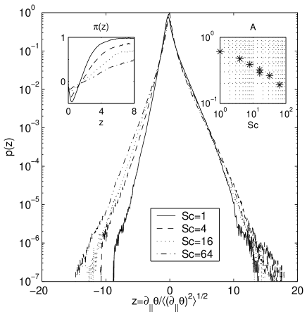
FIG. 1.: PDFs of the normalized longitudinal scalar derivative $z$ for $Sc$ = 1, 4, 16 and 64. The scalar has a mean gradient $G$ and is embedded in a Navier-Stokes velocity field, which is itself sustained by a constant mean gradient, $C$. The PDFs are shown in the main panel, and line styles in the legend. Left inset: the ratio $\pi(z)$. Right inset: the global asymmetry factor $A$ as a function of $Sc$. The decay of the derivative skewness, $\langle z^{3}\rangle$, with increasing $Sc$ is comparable to that in [1].

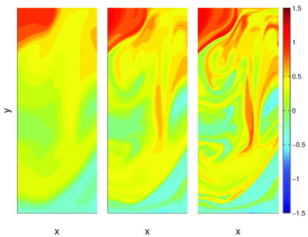
FIG. 2.: Slices of the total scalar field (mean plus fluctuation) for $Sc=1$ (left), 8 (middle), and 64 (right), all of which are advected by the same flow. Only a fraction of the simulation domain is shown.

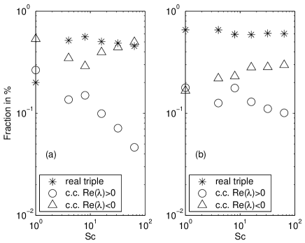
FIG. 3.: Fractions of eigenvalue triplets, as functions of $Sc$, in the vicinity of: (a) the steepest negative gradients, (b) steepest positive gradients.

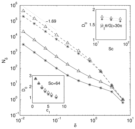
FIG. 4.: Box counting for scalar gradient sets $F$ for $Sc$ = 16 (solid lines) and 64 (dashed lines). The sets are defined by $|\partial_{\parallel}\theta/G|>30\pi$. Dotted lines indicate the range of scales for the fit. Exceeding nominal expectations, the scaling region is more extensive than the viscous-convective range (or the Batchelor regime). Triangles: positive gradients; asterisks: negative gradients. The differences between the $number$ of covering boxes for positive and negative gradients are larger for lower $Sc$ than for larger $Sc$. Upper right inset: Box counting dimensions fitted to the data of the main figure as a function of $Sc$. Lower left inset: Box counting dimension of a scalar gradient level set as a function of the threshold value, $c_{1}$, for $Sc=64$; here $z$ was taken within an interval $c_{1}\pm 0.025$. The symbols in insets are as in the main figure.

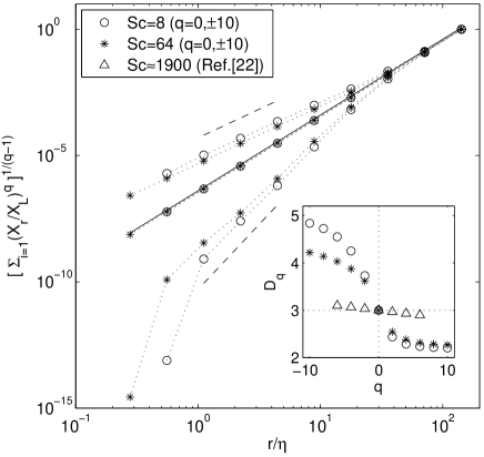
FIG. 5.: Multifractal analysis of the scalar dissipation field for $Sc=8$ and 64. Because all grid points are included, we have $D_{0}=3$, as indicated by the solid line. The dashed lines indicate the scaling range used to determine the $D_{q}$. The inset shows the spectrum of generalized dimensions, $D_{q}(q)$. Symbols for different $Sc$ are given in the legend.

REFERENCES

- [1] P. K. Yeung, S. Xu, and K. R. Sreenivasan, Phys. Fluids 14, 4178 (2002).
- [2] G. Brethouwer, J. C. R. Hunt, and F. T. M. Nieuwstadt, J. Fluid Mech. 474, 193 (2003).
- [3] K.R. Sreenivasan, Proc. Roy. Soc. Lond. 434, 165 (1991).
- [4] C. H. Gibson, C. A. Friehe, and S. O. McConnell, Phys. Fluids 20, S156 (1977); K. R. Sreenivasan, R. A. Antonia, and D. Britz, J. Fluid Mech. 94, 745 (1979); P. Mestayer, J. Fluid Mech. 125, 475 (1982); R. Budwig, S. Tavoularis, and S. Corrsin, J. Fluid Mech. 153, 441 (1985).
- [5] M. Holzer and E. D. Siggia, Phys. Fluids 6, 1820 (1994); ibid 7, 1519 (1995).
- [6] A. Pumir, Phys. Fluids 6, 2118 (1994).
- [7] A. Celani, A. Lanotte, A. Mazzino, and M. Vergassola, Phys. Fluids 13, 1768 (2001).
- [8] R. H. Kraichnan, Phys. Fluids 11, 945 (1968).
- [9] G. Falkovich, K. Gawȩdzki, and M. Vergassola, Rev. Mod. Phys. 73, 913 (2001).
- [10] M. Chertkov, G. Falkovich, and I. Kolokolov, Phys. Rev. Lett. 80, 2121 (1998).
- [11] E. Balkovsky and A. Fouxon, Phys. Rev. E 60, 4164 (1999); W. E and E. vanden-Eijnden, Physica D 152-153, 636 (2001); M. Chertkov and V. Lebedev, Phys. Rev. Lett. 90, 034501 (2003).
- [12] J. Schumacher, K. R. Sreenivasan, and P. K. Yeung, J. Fluid Mech. 479, 221 (2003).
- [13] G. K. Batchelor, J. Fluid Mech. 5, 113 (1959).
- [14] T. C. Halsey, M. H. Jensen, L. P. Kadanoff, I. Procaccia, and B. I. Shraiman, Phys. Rev. A 33, 1141 (1986).
- [15] K. R. Sreenivasan and C. Meneveau, Phys. Rev. A 38, 6287 (1988).
- [16] A. Brandenburg, I. Procaccia, D. Segel, and A. Vincent, Phys. Rev. A 46, 4819 (1992).
- [17] J. Schumacher, J. Fluid Mech. 441, 109 (2001).
- [18] K. J. Falconer, The Geometry of Fractal Sets, Cambridge University Press, Cambridge, 1986.
- [19] P. Constantin and I. Procaccia, Nonlinearity 7, 1045 (1994).
- [20] G. L. Eyink, Phys. Rev. E 54, 1497 (1996).
- [21] P. Grassberger, Phys. Lett. A 97, 227 (1983); H. G. E. Hentschel and I. Procaccia, Physica D 8, 435 (1983).
- [22] K. R. Sreenivasan and R. R. Prasad, Physica D 38, 322 (1989).
- [23] C. Meneveau and K. R. Sreenivasan, Phys. Rev. Lett. 59, 1424 (1987).