Exact Phase Solutions of Nonlinear Oscillators on Two-dimensional Lattice

Abstract

We present various exact solutions of a discrete complex Ginzburg-Landau (CGL) equation on a plane lattice, which describe target patterns and spiral patterns and derive their stability criteria. We also obtain similar solutions to a system of van der Pol’s oscillators.

1 Introduction

Near the onset of the Hopf bifurcation in continuous media, a complex amplitude of distributed oscillators is described by a normal form equation called the complex Ginzburg-Landau (CGL) equation. Some exact solutions of the 1+1 dimensional CGL equation are known as hole, solitary-wave and shock solutions [1]. In the 2+1 dimensional space, numerical studies showed existence of interesting solutions describing target patterns and spiral patterns [2, 3]. However, explicit and exact solutions representing target patterns or spiral patterns have not been constructed yet.

Here we consider a system of oscillators which undergo the Hopf bifurcation on a two dimensional lattice instead of continuous media. Each oscillator is governed by the normal form equation of the Hopf bifurcation [4] and couples diffusively and dispersively with its nearest-neighbor oscillators so that the system becomes a spatially discretized version of the 2+1 dimensional CGL (discrete CGL) equation[5]. Such a discrete CGL equation has also been studied on a network in connection with [7, 6]. In this paper, we show that the discrete CGL equation has exact solutions describing various phase patterns consisting of target patterns and spiral patterns. Each spiral pattern solution needs a defect in its origin of spiral, where oscillators are absent. This defect may corresponds to the singularity of the origin in a spiral solution in continuous media. In the other hand, target pattern solutions do not have any defects. We derive the stability condition of the exact solutions to modulational perturbations and conduct some numerical simulations to confirm the stability criterion. Similar phase pattern solutions are constructed to a system of van der Pol’s oscillators.

2 Nonlinear Oscillators on Two-dimensional Lattice

Let us consider the following system of normal form oscillators to the Hopf bifurcation on a two-dimensional lattice.

$$\frac{dW_{n}}{dt}=-(\mu_{r}+i\mu_{i})|W_{n}|^{2}W_{n}+(\nu_{r}+i\nu_{i})W_{n}+(\lambda_{r}+i\lambda_{i})\sum_{j\sim n}^{4}(W_{j}-W_{n})$$ (1)

where $W_{n}$ are complex amplitudes of oscillators and $\mu_{r},\ \mu_{i},\ \nu_{r},\ \nu_{i},\ \lambda_{r},\ \lambda_{i}$ are real constants; $\mu_{r}$ and $\nu_{r}$ are assumed to be positive (the subcritical bifurcation) and $\sum^{4}_{j\sim n}$ denotes summation over nearest-neighbor oscillators at site $n$. Through this summation term, each oscillator has diffusive ($\lambda_{r}$) and dispersive ($\lambda_{i}$) interactions with its nearest-neighbors. Here, we call Eq.(1) a discrete CGL equation.

By changing variables $W_{n}\rightarrow W_{n}\exp[-i\nu_{i}t]$ and $t\rightarrow\mu_{r}t$, and replacing coefficients as $p_{1}=\mu_{i}/\mu_{r}$, $p_{2}=\nu_{r}/\mu_{r}$, $p_{3}=\lambda_{r}/\mu_{r}$ and $p_{4}=\lambda_{i}/\mu_{r}$, Eq.(1) is transformed into

$$\frac{dW_{n}}{dt}=-(1+ip_{1})|W_{n}|^{2}W_{n}+p_{2}W_{n}+(p_{3}+ip_{4})\sum^{4}_{j\sim n}(W_{j}-W_{n}),$$ (2)

or

$$\frac{dW_{n}}{dt}=-(1+ip_{1})|W_{n}|^{2}W_{n}+(p_{2}-4(p_{3}+ip_{4}))W_{n}+(p_{3}+ip_{4})\sum^{4}_{j\sim n}W_{j},$$ (3)

where $p_{2}>0$. We use Eq.(2) or Eq.(3) as a basic system in this paper.

3 Exact Solutions

In this section, we derive some exact solutions of the discrete CGL equation (3), which represent a target pattern, a spiral pattern and various mixtures of those patterns. A crucial step to find exact solutions is to assume

$$\sum^{4}_{j\sim n}W_{j}=0\ \mbox{(for all sites}\ n\mbox{)}.$$ (4)

Then, Eq. (3) takes the same equation for all $n$:

$$\frac{dW_{n}}{dt}=-(1+ip_{1})|W_{n}|^{2}W_{n}+(p_{2}-4(p_{3}+ip_{4}))W_{n}.$$ (5)

We choose an equilibrium solution of Eq.(5).

$$W_{n}=Ae^{i(\omega t+\phi(n))},$$ (6)

where $A,\ \omega$ are real constants satisfying

$$A^{2} = p_{2}-4p_{3},$$ (7)

$$\omega = -p_{1}(p_{2}-4p_{3})-4p_{4},$$ (8)

and a functional form of the phase $\phi(n)$ with respect to $n$ is determined later. Because of $A^{2}>0$, we need

$$p_{2}-4p_{3}>0.$$ (9)

Since $p_{2}>0$, the condition (9) is automatically satisfied for $p_{3}\leq 0$ (negative diffusion or diffusionless case). The solution (6) has the same amplitude $A$ at all cites but its phase could vary from site to site. The variation of the phase must be determined so that Eq.(4) is satisfied.

$$\sum^{4}_{j\sim n}e^{i\phi(j)}=0\ \mbox{(for all sites}\ n\mbox{)}.$$ (10)

We consider a case that there are only two values for $\phi(n)$, that is, $\phi(n)=0$ or $\pi$. At every site, we set phase values of two oscillators among four nearest-neighbor oscillators as $\phi(n)=0$, while the other two phases are chosen to be $\pi$. Then, the condition (10) is fulfilled at all sites, that is,

$$\sum^{4}_{j\sim n}e^{i\phi(j)} = e^{i\cdot 0}+e^{i\cdot 0}+e^{i\cdot\pi}+e^{i\cdot\pi}$$ (11)

$$= 0\ \mbox{(for all sites}\ n\mbox{)}.$$

This choice of phase values is quite simple but produces a variety of phase patterns such as stripe patterns and target patterns as exact solutions. We can construct not only a single target pattern but also a combined pattern of some target patterns as shown in Fig.1. Although we present only a combined pattern of four target patterns, combined patterns of more or less target patterns are also possible. We can construct various combined patterns of target patterns indefinitely if the system size becomes larger.

When the lattice has a defect, that is, an oscillator is absent at a site, we should modify the above discussion for four oscillators around a defect. To four oscillators around a defect, the coupling terms in Eq.(2) are changed to

$$(p_{3}+ip_{4})\sum_{j\sim n}^{3}(W_{j}-W_{n}) = (p_{3}+ip_{4})(\sum_{j\sim n}^{3}W_{j}-3W_{n})$$ (12)

$$= (p_{3}+ip_{4})\left\{(W_{n}+\sum_{j\sim n}^{3}W_{j})-4W_{n}\right\},$$

where $n$ indicates one of the four oscillators and the summation term in Eq.(3) becomes

$$(p_{3}+ip_{4})(W_{n}+\sum_{j\sim n}^{3}W_{j}).$$ (13)

Thus, Eq.(10) is modified for each $n$-th oscillator around a defect as

$$e^{i\phi(n)}+\sum_{j\sim n}^{3}e^{i\phi(j)}=0.$$ (14)

Comparing Eq.(14) to Eq.(10), the term $\exp(i\phi(n))$ in (14) appears replacing the term which comes from an oscillator at a defect site. Therefore, for the $n$-th oscillator around a defect, the defect behaves as a mirror, that is, the defect acts as if it is an oscillator with the same phase as the $n$-th phase. Owing to this flexible property of a defect, we can construct spiral patterns with $2^{k}$ arms around $k\times k$ combined defects. For example, we obtain a spiral pattern with two arms around a single defect ($k=1$) and a spiral pattern with four arms around four combined defects ($k=2$) as shown in Fig.2 and Fig.4, respectively. Two separated defects produce two spiral patterns with the same or opposite rotation directions as shown in Fig.3. We can also construct various patterns in which spirals and targets are concurrent and show one of the simplest examples in Fig.2. On a large enough lattice, we could construct virtually an indefinite number of such spiral and target patterns.

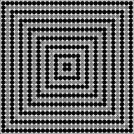
Figure 1: A target pattern. Black points denote $\phi(n)=0$, while gray points denote $\phi(n)=\pi$.

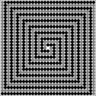
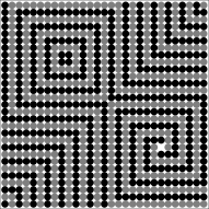
Figure 2: A spiral pattern with a defect and a combined pattern of a spiral and a target.

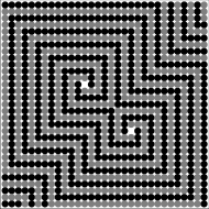
Figure 3: Two spiral patterns with the opposite and the same spiral rotations, respectively.

Figure 4: A four-arm spiral pattern and a two-arm spiral pattern

4 Stability of Solutions

Let us investigate a linear stability of the exact solution:

$$W_{n}^{0}(t)=Ae^{i(\omega t+\phi(n))}\ (\phi(n)=0\ \mbox{or}\ \pi),$$

$$\sum^{4}_{j\sim n}e^{i\phi(j)}=0\ \mbox{(for all site}\ n\mbox{)}.$$

Substituting a perturbed solution $W_{n}=W_{n}^{0}+\delta W_{n}$ into Eq.(3), we have

$$\frac{d}{dt}\delta W_{n} = i\omega\delta W_{n}-(1+ip_{1})A^{2}\delta W_{n}$$ (15)

$$-(1+ip_{1})A^{2}e^{2i(\omega t+\phi(n))}\delta W_{n}^{*}+(p_{3}+ip_{4})\sum^{4}_{j\sim n}\delta W_{j}.$$

As $\phi(n)=0$ or $\pi$, the coefficient of the third term in the RHS of Eq.(15) becomes $-(1+ip_{1})A^{2}\exp[i2\omega t]$, which does not depend on a site number $n$. Therefore, all coefficients of the linearized equation (15) are independent of $n$, which greatly simplifies stability analysis. Changing the variable as $\delta W_{n}\rightarrow\delta W_{n}\exp[-i\omega t]$, Eq.(15) is transformed into

$$\frac{d}{dt}\delta W_{n}=-(1+ip_{1})A^{2}(\delta W_{n}+\delta W_{n}^{*})+(p_{3}+ip_{4})\sum^{4}_{j\sim n}\delta W_{j}.$$ (16)

We consider plane-wave perturbations

$$\delta W_{n}=a(t)e^{i\vec{k}\cdot\vec{x}}=a(t)e^{i(k_{x}x+k_{y}y)},$$ (17)

where $\vec{x}=(x,y)$ indicates a lattice point and $\vec{k}=(k_{x},k_{y})$ is a wave-number vector. Then, the summation term of Eq.(16) reads

$$\sum^{4}_{j\sim n}\delta W_{j} = ae^{\vec{k}\cdot\vec{x}}(e^{ik_{x}}+e^{ik_{y}}+e^{-ik_{x}}+e^{-ik_{y}})$$

$$= ae^{\vec{k}\cdot\vec{x}}(2\cos k_{x}+2\cos k_{y})$$

$$= 2\delta W_{n}K,$$

where $K=\cos k_{x}+\cos k_{y}$. Hence, Eq.(16) reduces to

$$\frac{d}{dt}\delta W_{n} = -(1+ip_{1})A^{2}(\delta W_{n}+\delta W_{n}^{*})+2(p_{3}+ip_{4})K\delta W_{n}$$ (18)

$$= (2(p_{3}+ip_{4})K-(1+ip_{1})A^{2})\delta W_{n}-(1+ip_{1})A^{2}\delta W_{n}^{*},$$

or in terms of the real and imaginary parts of $\delta W_{n}$

$$\frac{d}{dt}\left(\begin{array}[]{c}\Re[\delta W_{n}]\\ \Im[\delta W_{n}]\end{array}\right)=2\left(\begin{array}[]{cc}p_{3}K-A^{2}&-p_{4}K\\ p_{4}K-p_{1}A^{2}&p_{3}K\end{array}\right)\left(\begin{array}[]{c}\Re[\delta W_{n}]\\ \Im[\delta W_{n}]\end{array}\right).$$ (25)

Eigenvalues of Eq.(25) are

$$2p_{3}K-A^{2}\pm\sqrt{-4p_{4}^{2}K^{2}+4p_{1}p_{4}A^{2}K+A^{4}}.$$ (26)

We denote an eigenvalue as $\alpha_{+}$ which has a larger real part than the other.

$$\alpha_{+}=2p_{3}K-A^{2}+\Re\left[p\sqrt{-4p_{4}^{2}K^{2}+4p_{1}p_{4}A^{2}K+A^{4}}\right].$$ (27)

If $\alpha_{+}\leq 0$ for any $K$ in $|K|\leq 2$, the various phase solutions are stable to a perturbation (17). For stability, $\alpha_{+}$ must take local maximum at K=0 since $\alpha_{+}=0$ at $K=0$ (see Fig.6, Fig.6). The derivative of $\alpha_{+}$ at $K=0$ is given as

$$\left.\frac{\partial\alpha_{+}}{\partial K}\right|_{K=0} = 2\left[p_{3}-p_{4}\frac{2p_{4}K-p_{1}A^{2}}{\sqrt{-4p_{4}^{2}K^{2}+4p_{1}p_{4}K+A^{4}}}\right]_{K=0}$$

$$= 2(p_{3}+p_{1}p_{4}).$$

A condition $p_{3}+p_{1}p_{4}=0$ is necessary for stability. When $p_{3}+p_{1}p_{4}=0$, we have

$$\left.\alpha_{+}\right|_{K=\frac{A^{2}}{2p_{3}}} = \Re\left[\sqrt{-\left(\frac{p_{4}}{p_{3}}\right)^{2}+2\frac{p_{1}p_{4}}{p_{3}}+1}\right]A^{2}$$

$$= \Re\left[\sqrt{-\left(\frac{p_{4}}{p_{3}}\right)^{2}-1}\right]A^{2}$$

$$= 0,$$

which shows that $K=A^{2}/2p_{3}$ is also a vanishing point of $\alpha_{+}$, where its derivative with respect to $K$ is finite. For stability, we need

$$|A^{2}/2p_{3}|\geq 2$$

or

$$A^{2}=p_{2}-4p_{3}\geq 4|p_{3}|,$$ (28)

Since $p_{2}>0$ is supposed, the condition (28) reads $p_{3}<0$ or $p_{2}>8p_{3}>0$.

Thus, we obtain the following conditions for our solutions to be stable.

$$p_{3}+p_{1}p_{4}=0$$ (29)

$$p_{3}<0\ \mbox{or}\ p_{2}\geq 8p_{3}>0.$$

\psfrag{a}[0.6]{$\alpha_{+}$}\psfrag{K}[0.6]{K}\includegraphics[width=142.26378pt]{pic5-1.eps} Figure 5: $\alpha_{+}(K)$ vs. $K$ for stable parameters ($p_{1}=-0.5$, $p_{2}=4.0$, $p_{3}=0.5$, $p_{4}=1.0$). \psfrag{a}[0.6]{$\alpha_{+}$}\psfrag{K}[0.6]{K}\includegraphics[width=142.26378pt]{pic5.eps} Figure 6: $\alpha_{+}(K)$ vs. $K$ for unstable parameters ($p_{1}=1.3$, $p_{2}=3.0$, $p_{3}=0.25$, $p_{4}=0.8$).

5 Numerical analysis of the system

First, we we conduct numerical analysis of the system with random initial perturbations in order to confirm validity of the stability condition (29). We set a boundary condition which enables our exact solutions to persist. It is supposed that, outside a boundary, there are oscillators whose phases are different from those just inside the boundary by $\pi$. This boundary condition is called a vanishing boundary condition in this paper. For values of parameters satisfying the stability condition (29), both target patterns and spiral patterns are found to be stable even for random perturbations. For example, in a stable case that $p_{1}=-0.5$, $p_{2}=4.0$, $p_{3}=0.5$ and $p_{4}=1.0$, a single target pattern and the pattern with two spirals are stable even for max $20\%$ random perturbations as shown in Fig.7.

Figure 7: Initial 20% random perturbations are added to exact solutions in a stable case that $p_{1}=-0.5,p_{2}=4.0,p_{3}=0.5,p_{4}=1.0$. Length of an arrow indicates $|W_{n}|$ and its direction means $\arg W_{n}$ .

\psfrag{amp}[0.6]{$|W|^{2}$}\psfrag{time}[0.6]{time}\includegraphics[width=142.26378pt]{pic8-2.eps}

Figure 8: A target pattern of the numerical solution at time $t=50$ for the initial condition given in Fig.7 and $|W_{n}|^{2}$ vs. $t$ for all $n$, which shows stability of the target pattern.

\psfrag{amp}[0.6]{$|W|^{2}$}\psfrag{time}[0.6]{time}\includegraphics[width=142.26378pt]{pic9-2.eps}

Figure 9: A combined spiral pattern of the numerical solution at time $t=50$ for the initial condition given in Fig.7 and $|W_{n}|^{2}$ vs. $t$ for all $n$, which shows stability of the combined spiral pattern.

Next, we show that a single target pattern can be reached from some initial conditions far from the exact solution. For example, setting initial values as $W_{n}=1/2,\ \phi(n)=\pi/4$ for all $n$ in the case $p_{1}=0.5$, $p_{2}=3.0$, $p_{3}=0.25$ and $p_{4}=-0.5$, we eventually have a target pattern, where $|W_{n}|=2$, shown in Fig.10. We also find other initial conditions far from the exact solution that lead to the single target pattern but those do not give enough informations for a basin structure of the target patterns.

Figure 10: An initial condition $|W|=0.5$ and phase$=\pi/4$ for all oscillators and a target pattern at time $t=150$ developed from the initial condition.

6 Van der Pol’s Oscillators

Similar exact target and/or spiral solutions can be also constructed for other diffusively and dispersively coupled systems of oscillators which undergo the subcritical Hopf bifurcation. For example, we consider a system of van der Pol’s oscillators which are coupled with each other diffusively and dispersively on a plane lattice.

$$\frac{d}{dt}x_{n} = y_{n}+ax_{n}-\frac{a}{3}x_{n}^{3}+D_{x}\sum^{4}_{j\sim n}(x_{j}-x_{n})$$

$$\frac{d}{dt}y_{n} = -x_{n}+D_{y}\sum^{4}_{j\sim n}(x_{j}-x_{n}),$$ (30)

where $a$ is a positive constant and $D_{x},D_{y}$ are diffusive and dispersive constants respectively. Let us seek phase solutions of Eq.(30) similar to those discussed earlier. Assuming

$$\sum^{4}_{j\sim n}x_{j}=0,$$ (31)

Eqs.(30) are reduced to a single van der Pol’s equation

$$\frac{d^{2}}{dt^{2}}X_{n}+(X_{n}^{2}-1)\frac{d}{dt}X_{n}+X_{n}=0,$$ (32)

where $\sqrt{1+4D_{y}}t\rightarrow t$, $x_{n}=(1-4D_{x}/a)^{1/2}X_{n}$ and

$$(1+4D_{y})>0,\quad(1-4D_{x}/a)>0$$ (33)

are assumed. If the van der Pol’s attractor of Eq.(32) is written as $x_{n}(t)=A(t)$, its opposite-phase function $x_{n}(t)=-A(t)$ is also the attractor of Eq.(32). By choosing $x_{n}(t)$ as $A(t)$ or $-A(t)$ for all $n$ so that $x_{n}(t)$ are satisfy the relation (31), we can construct various exact solutions whose phase patterns are exactly the same as those in the discrete CGL equation. However, the stability analysis will be much more difficult than the previous case.

7 Conclusions

We present various exact solutions of a discrete CGL equation on a plane lattice, which describe target patterns and spiral patterns and derive their stability criteria. Exact solutions obtained here represent not only a single target pattern and a single spiral pattern but also patterns consisting of targets and spirals. In the center of a spiral pattern, at least one defect is necessary and a number of spiral’s arms depends on a number of defects. For example, a defect produces a two-arm spiral and four defects in the center generate a four-arm spiral and so on. For a system of the van der Pol’s oscillators, we can also construct various exact solutions whose phase patterns are exactly the same as those in the discrete CGL equation. pp

References

- [1] K.Nozaki and N.Bekki, J. Phys. Soc. Jpn. 53 53 (1984), 1581.
- [2] I.S. Aranson, L. Aranson, L. Kramer, and A. Weber, Phys. Rev. A 46, R2992 (1992)
- [3] Igor S. Aranson and Lorenz Kramer, Rev. Mod. Phys. 74, 99 (2002)
- [4] J. Guckenheimer and P. Holmes, Nonlinear Oscillations,Dynamical Systems and Bifurcations of Vector Fields, Springer-Verlag (1983).
- [5] S. Mori: M. Thesis, Faculty of Science, Ochanomizu University, Otsuka, Bunkyo-ku, Tokyo, 1996.
- [6] H. Yamada and T. Nakagaki, talk at Traffic and Granular Flow ’01, October 15-71, 2001, Nagoya University, Japan.
- [7] S. H. Strogatz, Nature 410 (2001), 268.