Characterization of QPM gratings in $\chi^{(2)}$ media via second-harmonic-power measurements only

Abstract

A new scheme for non-destructive characterization of quasi-phase-matching grating structures and temperature gradients via inverse Fourier theory using second-harmonic-generation experiments is proposed. We show how it is possible to retrieve the relevant information via measuring only the power in the generated second harmonic field, thus avoiding more complicated phase measurements. The potential of the scheme is emphasized through theoretical and numerical investigations in the case of periodically poled lithium niobate bulk crystals.

I Introduction

Quasi-phase-matching or QPM is a major alternative over conventional phase-matching techniques in many laser applications based on frequency-conversion processes in nonlinear optical media (For reviews, see bye97 ; fejer98beamshaping ). With the maturing of QPM by periodic poling of LiNbO₃ (PPLN) webjorn94el ; hadi97josab ; baldi98oe it has become possible to produce more complicated QPM gratings simply by writing of the corresponding photo-lithographic mask fejer92jqe . This has led to a tremendous activity in engineered QPM gratings for applications in photonics.

A proper design of the longitudinal grating structure allows, e.g., for distortion free temporal pulse compression arbore97sepol , broad-band phase matching mizuuchi98ol , multi-wavelength SHG zhu97aprprl ; baldi95el , enhanced cascaded phase shiftcha98febol , and optical diodesgallo01julapl and gatesparameswaran00ptl . In high power schemes, QPM solitons are known to existfejer98beamshaping and longitudinal engineering can be used to tailor the solitonstorner98junol ; carrasco00sepol and to increase the bandwidth for their generationjohansen02oc . Transverse patterning can be used for beam-tailoring imeshev98mayol , broad-band SHG powers98ol , and soliton steering clausen98julprl ; clausen99janol .

Furthermore, nonuniform temperature distributions in the heated material may occur, leading to longitudinal dependent QPM conditions. This can result in a reduced nonlinear conversion efficiencychanvillard00apl or lead to positive effects such as a reduction of the fundamental-wave losses in cascaded phase shift configurationsschiek94ol .

The work presented here aims at characterizing these QPM structures in a non-destructive manner. The second-harmonic-generation process (SHG) has traditionally been the preferred choice in such attempts, since it requires only one tunable laser. By working in the low power regime, Fourier transform theory can be applied to retrieve the grating function. Until now the proposed methods have required the measurement of both the phase and the power in the generated SH field. Such methods are difficult to realize experimentally and it would be much more convenient if only the power was required. This is indeed what we propose here. By utilizing a mirror in the setup we show how it is possible, in principle at least, to obtain all relevant information via easily performed power-only measurements.

We start by developing the general Fourier scheme with arbitrary choice of mirrors in section II. Afterwards we apply the scheme to the concrete case of PPLN. In section IV we focus on determining the grating function. This can be done at room temperature because we operate in the low power regime, i.e. we can neglect photo-refractive effects. When heated the temperature distribution along the crystal may become nonuniform and the determination of such temperature profiles is the subject of section V. Throughout the paper we have made an effort to ensure that the numerical simulations are in agreement with the parameter settings which will be encountered in the laboratory.

II Theoretical description of the inverse method

We consider type-I SHG in a lossless QPM $\chi^{(2)}$ crystal. The evolution along the propagation direction $z$ of the normalized slowly varying envelopes $E_{1}=E_{1}(z)$ and $E_{2}=E_{2}(z)$ at the fundamental pump wavelength $\lambda_{p}$ (FW) and at the second harmonic wavelength $\lambda_{s}=\lambda_{p}/2$ (SH), respectively, is governed by

$$i\frac{\partial E_{1}}{\partial z}+d(z)E_{1}^{*}E_{2}\exp\left(-i\int_{0}^{z}\beta(z^{\prime})\>\mbox{\small d}z^{\prime}\right)=0,$$ (1)

$$i\frac{\partial E_{2}}{\partial z}+d(z)E_{1}^{2}\exp\left(i\int_{0}^{z}\beta(z^{\prime})\>\mbox{\small d}z^{\prime}\right)=0.$$ (2)

The wave vector mismatch, the so called phase mismatch, is introduced through $\beta(z)=4\pi(n_{1}-n_{2})/\lambda_{p}$ where $n_{1}=n_{1}(\lambda_{p},T)$ and $n_{2}=n_{2}(\lambda_{s},T)$ are the wavelength and temperature dependent refractive indices in the crystal experienced by the FW and the SH, respectively. The refractive indices and hence the phase mismatch $\beta$ can be estimated via Sellmeier fits. For bulk PPLN the temperature-dependent Sellmeier equationjundt97octol reads

$$n^{2}=a_{1}+b_{1}f+\frac{a_{2}+b_{2}f}{\lambda^{2}-(a_{3}+b_{3}f)^{2}}+\frac{a_{4}+b_{4}f}{\lambda^{2}-a_{5}^{2}}-a_{6}\lambda^{2},$$ (3)

where the wavelength $\lambda$ is measured in $[\lambda]=\mu\mbox{m}=10^{-6}\mbox{m}$ and the temperature $T$ is expressed in degrees Celsius with the temperature parameter $f$ given by

$$f=(T-{24.5\>}^{\circ}C)(T+{570.82\>}^{\circ}C).$$ (4)

Variations in the second order susceptibility $\chi^{(2)}$ due to the imposed grating is accounted for through the grating function $d(z)$, i.e. ${\chi^{(2)}}(z)=d(z)\chi^{(2)}_{int}$. $\chi^{(2)}_{int}$ is the intrinsic strength of the largest second order susceptibility coefficient exploited in QPM configurations which for lithium niobate is $\chi^{(2)}_{int}=d_{33}\sim 30p\mbox{m}/V$. Furthermore, in experiments the crystals are often heated to eliminate photo-refractive effects. The heating is in general nonuniform and therefore the phase mismatch becomes $z$-dependent through $T=T(z)$.

The real and measurable powers $P_{1}$ and $P_{2}$ at the FW and at the SH, respectively, are via the normalization given by

$$P_{1}=\eta A|E_{1}|^{2},\qquad P_{2}=2\eta A|E_{2}|^{2},$$ (5)

where $\eta(\lambda_{p},T_{0})=\frac{n_{1}^{2}n_{2}\lambda_{p}^{2}}{4\pi^{2}\eta_{0}d_{33}^{2}}$. $\eta_{0}$ is the impedance of free space and $A$ is the cross area of the Gaussian pump beam. We emphasize that for normal temperature variations, i.e. $\pm 10^{\circ}\mbox{C}$, the variations in the refractive indices are small. Hence $\eta$ can be assumed to depend only on $\lambda_{p}$ and a reference temperature $T_{0}$ which we take to be the temperature at the beginning of the crystal. We also note that because of the way we have chosen to normalize the system we measure $\eta$ in Watts, i.e. $[\eta]=\mbox{W}$, and $E_{j}$ in reciprocal meters, i.e. $[E_{j}]=\mbox{m}^{-1}$. This normalization allows us to operate with the relevant physical parameters, i.e. the wavelengths, the grating period, the phase mismatch, and the temperature, while preserving a simple structure in the governing equations.

As described in the introduction, we aim at solving the inverse problem, i.e. to determine the grating function $d(z)$, knowing only the input powers at both wavelengths and the output power of the SH. Solving Eq. (1-2) for $d(z)$ in principle requires information on both the input and output amplitude at both wavelengths and the relative phases. The problem is significantly reduced by assuming that the FW is undepleted in which case the solution can be found by applying the inverse Fourier transformation on Eq. (2). To simplify the argument we keep the temperature uniform for the moment and launch only FW. The normalized SH intensity at the output of the crystal is then given by

$$|E_{2}(\beta,L)|^{2}=|E_{1}^{2}(0)|^{2}\mathcal{F}\{\tilde{d}(z)\}\mathcal{F}^{*}\{\tilde{d}(z)\},$$ (6)

where $\tilde{d}(z)=u(z)d(z)$ is the grating function modified with the window function $u(z)$ which is 1 if $0<z<L$ and 0 otherwise, with $L$ being the length of the crystal. The complex Fourier transform has been defined as $\mathcal{F}\{f(z)\}=\int_{-\infty}^{\infty}f(z)\exp(-i\beta z){\mbox{d}}z$ and $\mathcal{F}^{*}\{f(z)\}$ denotes its conjugated. In general we do not know any of the symmetry properties of the grating function, except that it is real, and hence we cannot hope to determine the grating function from Eq.(6) knowing only the power spectrum of the SH alone; additional phase information is required. However, we observe that if we could force the grating function to be even then by virtue of symmetry properties the Fourier transform would become real and in principle Eq.(6) could then be solved without the phase information.

Figure 1: Illustration of how to generate an even grating function with the help of a mirror.

One way in which we can force the grating function to be even, is to put a mirror directly at the output surface of the QPM crystal. Mathematically speaking we simply prolong the original grating function with its mirror image and let this new grating function of length $2L$ enter as $d(z)=d(-z)$ in Eq.(2). Naturally any temperature distribution would likewise become an even function in $z$. In Fig. 1 we have sketched the situation with the emphasis on the point that $d(z)$ is now both even and real; the prerequisite for solving the problem via inverse Fourier transformation.

Before Eq. (2) is integrated in the general case with a grating and nonuniform temperature profile, we need to elaborate a bit more on the mirror. In general the waves are affected in two ways by the mirror: they experience a phase shift and they are attenuated. Though we shall later focus on metallic mirrors where both wavelengths experience a $\pi$ phase shift, we here set up more general mirror conditions since other mirrors such as dielectric ones might be of interest. At the mirror we have

$$E_{j}(\hat{z}=0^{+})=r_{j}\exp(im_{j})E_{j}(\hat{z}=0^{-}),\qquad j=1,2,$$ (7)

where $r_{j}$ and $m_{j}$ are the amplitudes and the phase shifts, respectively, of the reflection coefficients. The reflection coefficients are in general wavelength dependent.

We can now perform the integration of Eq.(2) in the general case of a grating function $d(z)$ and a nonuniform temperature profile. The result is

$$E_{2}(L)=r_{2}e^{im_{2}}E_{2}(-L)$$

$$\quad+i[r_{1}^{2}e^{i2m_{1}}+r_{2}e^{im_{2}}]E_{1}(-L)^{2}\int_{0}^{L}d(z)\left[\cos B\cos(\beta_{0}z)-\sin B\sin(\beta_{0}z)\right]{\mbox{d}}z$$

$$\quad-\;[r_{1}^{2}e^{i2m_{1}}-r_{2}e^{im_{2}}]E_{1}(-L)^{2}\int_{0}^{L}d(z)\left[\cos B\sin(\beta_{0}z)+\sin B\cos(\beta_{0}z)\right]{\mbox{d}}z.$$ (8)

For simplicity we have set $B(z)=\int_{0}^{z}\delta\beta(z^{\prime})\>{\mbox{d}}z^{\prime}$ where $\delta\beta(z)=4\pi[\delta n_{1}(t(z))-\delta n_{2}(t(z))]/\lambda_{p}$ is the $z$-dependent part of the phase mismatch $\beta(\lambda_{p},T)=\beta_{0}(\lambda_{p},T_{0})+\delta\beta(t(z))$ with the reference temperature $T_{0}$ at the beginning of the crystal and total temperature $T(z)=T_{0}+t(z)$ at the coordinate $z$. Henceforth we shall refer to $t(z)$ as the temperature profile. $\delta n_{j}(t(z))$ is the $z$-dependent part of the total refractive index $n_{j}(T_{0},\lambda_{p},t(z))=n_{0,j}(T_{0},\lambda_{p})+\delta n_{j}(t(z))$ determined from Eq. (3).

Eq.(8) is the starting point for all further analysis in this paper and in the next section we show how it applies to the case of a metallic mirror. Here, however, we feel that we must supply a few general comments on the structure of the integrals in Eq.(8) which eventually will be solved by applying Fourier theory. The way we have set up Eq.(8) indicates that we have chosen the $z$-independent part of the phase mismatch, $\beta_{0}$, and the coordinate $z$ to be our Fourier variables. In an experimental situation we have the option of changing $\beta_{0}$ through either of the two independent variables, i.e. through the pump wavelength $\lambda_{p}$ or through the reference temperature $T_{0}$. It is clear that application of Fourier’s integral theorem to any of the integrals in Eq.(8) requires that the function $B$ must be independent of $\beta_{0}$ or more specifically: $B$ must be independent of the independent variable through which we change $\beta_{0}$. Since $B$ depends explicitly on $\lambda_{p}$ through the way we have defined $\delta\beta$ above, we can immediately rule out to determine temperature profiles by changing $\beta_{0}$ through the wavelength. Hence temperature profiles must be determined by changing $\beta_{0}$ through temperature. In theory this requires that $\delta n_{j}(t(z))$ be independent of $T_{0}$ and in section V we show that for small variations in temperature this can indeed be assumed to be so. The same assumption has been applied on waveguides in PPLNschiek98nlgw and thus the theory presented here is applicable for other materials and experimental setups.

Once the mirror type has been decided on Eq.(8) is readily solved even if it looks complicated. We notice that by proper engineering of the mirror we can make either the sum or the difference between the two reflection amplitude coefficients in Eq.(8) vanish. It is this fact that allows us to simplify Eq.(8). Put differently we can state that because of the spatial symmetries of the mirror-expanded grating function, which forces the involved Fourier integrals to be real, it is essentially no longer necessary to obtain the phase information that we need in order to solve Eq. (6).

III Modeling with a metallic mirror in bulk lithium niobate

We now focus on exploiting metallic mirrors. These mirrors are relatively cheap and can be produced with reflection amplitude coefficients very close to 1. Though the coefficients are wavelength dependent, it is reasonable to assume that $r_{1}\sim r_{2}$ and that they vary little around each of the wavelengths. With both waves experiencing a $m_{j}=\pi$ phase shift, the sum between the reflection amplitude coefficients in Eq. (8) vanishes and the unseeded normalized SH output intensity as found from Eq. (8) becomes

$$|E_{2}(\beta_{0},L)|^{2}\approx\left(r_{1}^{2}+r_{2}\right)^{2}E_{1}(-L)^{4}f^{2}(\beta_{0}),$$ (9)

where $f(\beta_{0})=\int_{0}^{L}d(z)\left[\sin B\cos(\beta_{0}z)+\cos B\sin(\beta_{0}z)\right]{\mbox{d}}z$. From Fourier’s integral theorem we then know that

$$\tilde{d}(z)\cos B=\frac{2\mathcal{F}_{IM}^{-1}\left\{E_{2}(L)\right\}}{(r_{1}^{2}+r_{2})E_{1}(-L)^{2}},\quad\tilde{d}(z)\sin B=\frac{2\mathcal{F}_{RE}^{-1}\left\{E_{2}(L)\right\}}{(r_{1}^{2}+r_{2})E_{1}(-L)^{2}},$$ (10)

where $\mathcal{F}_{IM}^{-1}$ and $\mathcal{F}_{RE}^{-1}$ are the imaginary and real part, respectively, of the inverse Fourier transform. Again $\tilde{d}(z)$ is the grating function modified with the window function $u(z)$ according to $\tilde{d}(z)=u(z)d(z)$ where $u(z)=1$ if $0<z<L$ and 0 otherwise. With no temperature profile present, $B=0$, and $f(\beta_{0})$ becomes an odd function in $\beta_{0}$. Hence we can apply the inverse Fourier sine transform, $\mathcal{F}_{s}^{-1}\{f(\beta_{0})\}=\frac{2}{\pi}\int_{0}^{\infty}f(\beta_{0})\sin(\beta_{0}z){\mbox{d}}\beta_{0}$, and determine the grating function through

$$\tilde{d}(z)=\frac{\mathcal{F}_{s}^{-1}\{E_{2}(L)\}}{(r_{1}^{2}+r_{2})E_{1}(-L)}=\frac{\sqrt{A}}{\sqrt{2}(r_{1}^{2}+r_{2})P_{1,I}}\mathcal{F}_{s}^{-1}\left\{\sqrt{\eta P_{2,O}}\right\}.$$ (11)

$P_{2,O}$ and $P_{1,I}$ are the measured SH output power and the FW input power, respectively, as given by Eq. (5). We notice that both $\eta$ and $P_{2,O}$ are functions of $\beta_{0}$ and that the inverse sine transform must be applied to the product of the two functions.

In principle we can now determine any grating function in a uniform temperature distribution simply by measuring the SH output power as a function of the pump wavelength; additional phase information is no longer required. The attentive reader will have noticed that the arguments of the inverse Fourier transforms in Eq. (10) should have been functions of the absolute value of the SH field $|E_{2}(L)|$ instead of just the real value $E_{2}(L)$. Of course $|E_{2}(L)|$ is what we measure but we need the sign information to correctly reconstruct the grating function and temperature profile. Luckily the sign information is easily retrieved by exploiting that the derivative of $E_{2}(L)$ with respect to $\beta_{0}$ must be a smooth function in $\beta_{0}$ whereas the derivative of $|E_{2}(L)|$ is not. Whenever the sign of $E_{2}(L)$ changes we get non-analytical points in the derivative of $|E_{2}(L)|$ with respect to $\beta_{0}$. These points can be located numerically and hence $E_{2}(L)$ can be determined.

IV Simulation results: Determining the grating function

In the following we present simulation results validating Eq. (11) and we discuss the determination of the grating function in uniform temperature profiles. As mentioned above we are now, because of the mirror, able to reconstruct any grating function simply by measuring the SH output power $P_{2,O}$ as a function of pump wavelength. In this section we shall first verify Eq. (11) with simulations on a perfectly periodic QPM crystal, i.e. we show that the contribution from the first integral in Eq. (8) is negligible even if we have considerable mirror losses in the setup. Secondly we shall focus on the case of a perfectly periodic crystal with a duty-cycle different from $D=0.5$. This example clearly illustrates the differences between the same experiments made with and without the mirror and hence emphasizes the strength of the presented scheme. The last part of this section is dedicated to a discussion of the limitations of the presented scheme. We remark that these limitations are not a consequence of not making phase measurements but rather an inherent problem of applying Fourier theory to the particular case of determining QPM gratings in periodically poled materials.

We leave the determination of temperature gradients to the next section and set $T(z)=24.5$ in Eq. (3) in the following. With a pump laser tunable in the interval $\lambda_{p}\in[1.5\mu\mbox{m}\;1.6\mu\mbox{m}]$ this yields phase mismatches in the approximate range $\beta_{0}\in[-3.6\times 10^{5}\mbox{m}^{-1}\;{-3.0\times 10^{5}\mbox{m}^{-1}}]$. In a traditional domain inverted QPM crystal this corresponds to a domain length of $\sim 10\mu\mbox{m}$ or around $10\,000$ domains in a 1$c\mbox{m}$ long crystal. Possibly the crystals we want to characterize are several centimeters long. With a beam diameter of $350\mu\mbox{m}$ the cross area of the Gaussian pump beam is $A=9.62\cdot 10^{-8}\mbox{m}^{2}$ and the wavefront can be assumed planar for approximately $10c\mbox{m}$. With a pump power of $10m\mbox{W}$ this yields a FW intensity of $I_{1}\sim 100\,000\mbox{W}/\mbox{m}^{2}$. To establish whether this intensity is in the low-depletion regime we use the analytical solution at perfect phase matching for SHG with first order QPMarmstrong62pr . For propagation distances less than $9c\mbox{m}$ we get that the FW is unaltered to within $1\times 10^{-4}$ of its initial value. The numerical results confirm that this is indeed in the low depletion regime. Regarding the detection of the SH output we shall here assume that we can measure 0.1$n$W and numerically put all values below that to zero. In the following we refer to this value as the cut-off on the SH power measurement.

IV.1 Determination of domain length in perfectly periodic crystal

To illustrate the method and to verify it in the presence of mirror losses we here consider the case of determining the domain length in a perfectly periodic crystal with a duty-cycle $D=0.5$, i.e. the domain length is the same for the $d=-1$ and $d=1$ domains. The grating function can be expanded according to

$$d(z)=\left\{\begin{array}[]{rl}1,&\;0<z<\Lambda\\ -1,&\;\Lambda<z<2\Lambda\end{array}\right.=\frac{4}{\pi}\sum_{n=1,3,5,--}\frac{\sin(nz\pi/\Lambda)}{n}.$$ (14)

Choosing first order QPM, i.e. $n=1$ in Eq. (14), we can rewrite Eq. (9) and express the output SH power as

$$P_{2}\approx\frac{8}{\pi^{2}}\frac{\left(r_{1}^{2}+r_{2}\right)^{2}L^{2}}{A\eta}P_{1}^{2}\mbox{sinc}^{2}\left[\left(\frac{\pi}{\Lambda}+\beta_{0}\right)L\right],$$ (15)

where $\mbox{sinc}(x)=\sin x/x$.

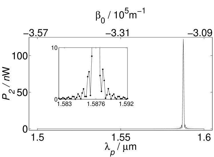
Figure 2: SHG tuning curve for perfectly periodic QPM crystal of length $L=1c\mbox{m}$ and with domain length $\Lambda=10\mu\mbox{m}$. The reflection amplitude coefficients of $r_{1}=0.95$ and $r_{2}=0.75$. The curve is in fact discrete which is indicated with dots in the enlarged part of the curve shown in the inset.

In Fig. 2 we show the tuning curve found from a numerical experiment on a $1c\mbox{m}$ long crystal with a domain length of $1\times 10^{-5}\mbox{m}$. In the simulation we have used reflection amplitude coefficients of $r_{1}=0.95$ and $r_{2}=0.75$ for the FW and the SH, respectively. The reflection amplitude coefficients have been chosen so that the difference between them is sufficiently big to encompass any differences we imagine could be encountered in the laboratory. Finally we assume that the laser shares the above discussed characteristic with a FW power of $P_{1}=10m\mbox{W}$ and scan through the pump wavelength interval with a step-length of $\Delta\lambda_{p}=2\times 10^{-10}\mbox{m}$ which yields a total of 500 measurements.

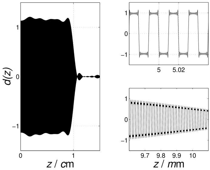
Figure 3: Reconstructed grating function from the SHG tuning curve in Fig. 2. The entire grating function is shown to the left. Two enlarged parts of the grating is shown to the right: The middle part in the top and the part around the end of the crystal in the bottom.

It is well knownarmstrong62pr that we would also get a sinc-shaped tuning curve from the corresponding no-mirror case and that the phase information likewise is not needed to reconstruct the actual grating function. The numerical experiment in Fig. 2 is non-trivial because it shows that we can apply the approximation given in Eq. (9), i.e. that the scheme works even for considerable mirror losses. In fact, we have put the theoretical curve as found from Eq. (15) on top of the curve in Fig. 2 and the experimental points fall on the curve to within the precision inherent to the Fourier transform and to within the precision owing to the cut-off on the SH power measurement.

To recover the grating function we need to generate the full tuning curve spanning the entire $\beta_{0}$-axis, thus covering all the QPM peaks owing to the different QPM orders. Numerically speaking, however, we only need to take into account the first few peaks and here we have chosen to work with the 7 first higher order peaks, making the computational effort tolerable. The expansion of the tuning curve is fairly trivial in the case of the perfectly periodic duty-cycle $D=0.5$ crystal. First we locate the maximum of the tuning curve on the $\beta_{0}$-axis. Once we know the location $\beta_{0,max}$ of the maximum, then Eq. (15) tells us that the $n$’th order peak is located at $\beta_{0}=n\beta_{0,max}$. We remark that the $\beta_{0}$-axis and the $\lambda_{p}$-axis in Fig. 2 are connected through the Sellmeier Eq. (3) and we notice how the absolute value of $\beta_{0}$ here is a decreasing function in $\lambda_{p}$. Hence on the $\lambda_{p}$-axis the higher order QPM peaks are located closer to $\lambda_{p}=0$ whereas they are located at numerically higher values of $\beta_{0}$ than the maximum value on the $\beta_{0}$-axis. The series of experiments is performed keeping the step-length $\Delta\lambda_{p}$ constant. Since the Sellmeier equation is nonlinear the step-length $\Delta\beta_{0}$ on the $\beta_{0}$-axis will not be constant and numerical routines must be supplied to fix this problem. We can estimate the resolution in the $z$-domain, i.e. the inverse Fourier domain, through $\Delta z=2\pi/(\Delta\beta_{0}\times\beta_{0,disc})$, where $\beta_{0,disc}$ are the total number of experiments. By using the shortest step-length we find on the original $\beta_{0}$-axis we get an estimate on the coarsest resolution we can expect yielding $\Delta z\sim 1.6\mu\mbox{m}$ which is good enough to resolve domain lengths on the order of 10$\mu\mbox{m}$.

We are now ready to apply Eq. (10) and perform the inverse Fourier transform. The result is shown in Fig. 3. The figure shows both the complete recovered function and two enhancements: one of the middle part and one of the part around the end of the crystal. The figure showing the complete recovered function is entirely black owing to the fact that the value of $d(z)$ changes $10\;000$ times in the interval $z\in[0\;1c\mbox{m}]$. From the enhanced part of the grating function from the middle of the crystal we observe that the domain length is correctly retrieved. The small oscillations around $d(z)=\pm 1$ are due to the inherent difficulties in making numerical Fourier transforms and can only be reduced by enhancing the resolution. On the other hand the oscillations are not critical in the case of PPLN since we now that $d(z)=\pm 1$ and cannot take any values in between. Somewhat more critical is the fact that we according to the close up of the part around the end of the crystal do not get a nice sharp cut at $z=1c\mbox{m}$. Instead we get a slow decrease in the value of $d(z)$ which eventually becomes zero as can be seen from the figure showing the entire grating function. We have verified that the problems in correctly retrieving the grating function around the end of the crystal are due to the cut-off on the SH power measurement. With a lower cut-off the grating function goes to zero within very few oscillations.

In conclusion we can say that with no cut-off on the SH power measurement and with indefinite resolution the grating would off course have been perfectly retrieved. On the other hand this is what we would expect from experiments like this and as such it is not a consequence of the scheme we propose, i.e. experiments made with no mirror by measuring the phase instead would be subject to the same difficulties. Thus we have verified that the scheme is applicable even with mirror losses, or more precisely: with a considerable difference between the loss experienced in the FW and that experienced in the SH.

IV.2 duty-cycle errors

We now turn towards an example which demonstrates how our scheme immediately renders information which would otherwise require phase measurements. In the previous part we investigated the perfectly periodic QPM crystal with a duty-cycle $D=0.5$. Here we shall still consider only perfectly periodic crystals but with arbitrary duty cycle, $D\in[0.5\;1]$. Such a grating function can be expanded in the Fourier series

$$d(z) = \left\{\begin{array}[]{rl}1,&\;0<z<2D\Lambda\\ -1,&\;2D\Lambda<z<2\Lambda\end{array}\right.$$ (19)

$$= -2\left(\frac{1}{2}-D\right)+\frac{4}{\pi}\sum_{n=1,3,--}\frac{\sin(n\pi/2)\sin(nD\pi)}{n}\sin\left[n\frac{\pi}{\Lambda}z+n\pi\left(\frac{1}{2}-D\right)\right]$$

$$\qquad+\frac{4}{\pi}\sum_{n=2,4,--}\frac{\sin((n+1)\pi/2)\sin(nD\pi)}{n}\sin\left[n\frac{\pi}{\Lambda}z+n\pi\left(\frac{1}{2}-D\right)\right].$$

The problem can still be solved analytically and for the SH output at the first order QPM peak, $n=1$ in Eq. (19), Eq. (9) reduces to

$$P_{2} \approx \frac{8}{\pi^{2}}\frac{\left(r_{1}^{2}+r_{2}\right)^{2}L^{2}}{A\eta}P_{1}^{2}\sin^{2}\left(D\pi\right)\left[\frac{\cos\left[q-\pi D\right]-\cos\left(\pi D\right)}{q}\right]^{2},$$ (20)

where for simplicity we have set $q=\left(\frac{\pi}{\Lambda}+\beta_{0}\right)L$. We observe that for $D=0.5$ Eq. (20) reduces to Eq. (15). For $D\neq 0.5$ we see that the solution (20) is scaled by a factor $\sin^{2}(D\pi)$. The solution is also no longer sinc shaped as compared to Eq. (15) and this is an important observation. In a normal setup, i.e. without utilizing a mirror, the solution would indeed still have been sinc shapedfejer92jqe making it difficult to distinguish from the duty-cycle $D=0.5$ solution. Of course it would still be scaled by the factor $\sin^{2}(D\pi)$ but since we would like to determine both the duty cycle, $D$, and the domain length, $\Lambda$, additional phase information would still be required. In our scheme, however, this is not so.

In Fig. 4 we have shown the outcome of an experiment where the duty-cycle $D\neq 0.5$. All other parameters are the same as the ones used to produce Fig. 2. If we compare Fig. 2 and Fig. 4 there is an obvious difference in the shape around the central peaks. Suppose we did not know anything about the crystal in front of us, then because of the asymmetric tuning curve in Fig. 4 we can immediately conclude that either the crystal is not perfectly periodic or the duty-cycle $D\neq 0.5$. Since we do not know the tuning curve throughout the entire $\beta_{0}$-axis, we have to make assumptions in order to further characterize the grating function responsible for the tuning curve. Duty-cycle errors are not uncommon and hence it would be a reasonable starting point to assume that we are dealing with exactly that, then perform the analysis, and then verify the nature of the error by simply holding it up against the theoretical solution.

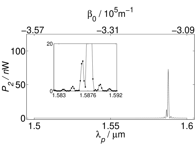
Figure 4: SHG tuning curve for periodic QPM crystal with duty-cycle $D=0.7$. The other parameters are the same as for Fig. 2.

In order to determine the duty-cycle and the domain length we need to measure two things in Fig. 4: the maximum value, $P_{2,max}$, of the generated SH and its location, $\beta_{0,max}$, on the $\beta_{0}$-axis. The maximum value $P_{2,max}$ is independent of where on the $\beta_{0}$-axis it is located and hence we can determine the duty-cycle as a function of $P_{2,max}$. Knowing $D$ we can also find $q_{max}$ which is determined through the transcendental equation

$$q=\frac{\sin\left(\frac{q}{2}\right)\sin\left(\frac{q}{2}-\pi D\right)}{\sin\left(q-\pi D\right)}.$$ (21)

Since we have measured $\beta_{0,max}$ and $q_{max}=\left(\frac{\pi}{\Lambda}+\beta_{0,max}\right)L$ we can now easily retrieve the domain length $\Lambda$. In Fig. 5 we have sketched how we determine the duty cycle and domain length with the letters indicating the order discussed above. The point at ’A’ indicates $P_{2,max}$ which we have measured on Fig. 4 to be $P_{2,max}\approx 78n\mbox{W}\Rightarrow p\approx 0.6$ where $p=P_{2,max}/P_{2,max}(D=0.5)$, i.e. $p$ is the maximum output power relative to the maximum of Fig. 2. Following the line to point ’B’ we determine the duty-cycle to be $D\approx 0.70$. We then jump to point ’C’ on the curve showing the domain length as a function of the duty-cycle. Following the line to point ’D’ finally gives us the domain length $\Lambda\approx 10.000\mu\mbox{m}$.

The method outlined above does not involve Fourier transformation since we have already made assumptions as to the nature of the grating function. To verify if we are indeed dealing with duty-cycle errors and that we have found the right values for the duty-cycle and the domain length we only have to put the analytical solution (20) on top of the curve in Fig. 4 and see if it fits. We emphasize that without using the mirror setup, it is necessary also to measure the phase of the SH in order to apply the method illustrated by Fig. 5.

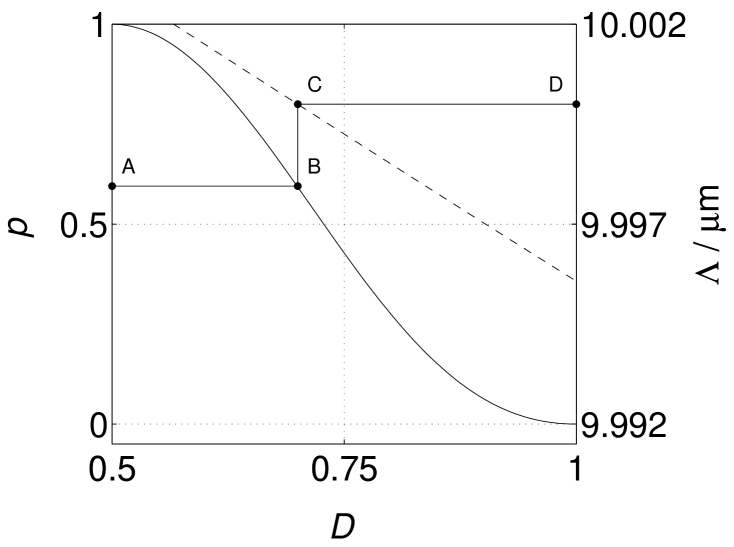
Figure 5: Determination of duty-cycle $D$ and domain length $\Lambda$ in the presence of duty-cycle errors. The full curve shows the maximum relative SH output power $p=P_{2,max}/P_{2,max}(D=0.5)$ as a function of $D$. The dashed line shows $\Lambda$, also as function of $D$, determined via Eq. 21). See text for explanation of the letters A, B, C, and D.

IV.3 Discussion on the limitations of the inverse method

We shall keep this discussion on the limitations of the inverse method short since these are a consequence of the nature of the Fourier transform rather than due to the here proposed scheme with the mirror setup.

Essentially the biggest hurdle for the inverse method is the limited $\beta_{0}$-bandwidth owing to the limited wavelength range for the used lasers. This is of course connected to the fact that using PPLN moves the central peak on the tuning curve far away from $\beta_{0}=0$ which means that the $\beta_{0}$-bandwidth in practice must be huge to encompass all the information of the SH tuning curve. Even if we had an unlimited wavelength range it is doubtful if we could go all the way to $\beta_{0}=0$. This is evident from for instance the Sellmeier Eq. (3) we here apply for bulk PPLN.

With a limited $\beta_{0}$-bandwidth far away from zero we can in theory only hope to characterize a limited category of grating functions, namely those which are periodic and for which the corresponding Fourier frequencies falls within the $\beta_{0}$-bandwidth. Aperiodic functions in general have dense Fourier spectra and hence we would not be able to get all the necessary information to retrieve the grating function. In a traditional setup with no mirror grating functions with stochastic boundary errors, with missing domain reversals or with single domains of different length like the optical diodegallo01julapl are all knownfejer92jqe to share the familiar sinc-shape and as such they are indistinguishable from the perfectly periodic crystal. Only when the relative sizes of the errors become sufficiently large compared to the domain length, they change the shape of the sinc significantly. The situation does not change even if we use the mirror setup. The big problem is that the information from these aperiodic errors is not folded around the QPM peaks but rather around $\beta_{0}=0$, far away from any realizable $\beta_{0}$.

Once again we emphasize that the above limitations will always be present, mirror or not. However, as exemplified above for duty-cycle errors, the mirror setup allows for power-measurement-only characterization of periodic functions which are bandwidth limited to within the realizable $\beta_{0}$-interval. We have verified that the scheme can also be applied to the case of a linear increase in the domain length.

V Simulation results: Measuring temperature profiles

We now turn towards experimental conditions where a temperature profile, $t(z)$, is present. In Fig. 6 we have sketched such a situation emphasizing how the temperature profile, like the grating function, becomes an even function in $z$ when utilizing the mirror setup.

Figure 6: QPM crystal in mirror setup illustrating the even mirror-expanded temperature profile, $t(z)$.

As discussed in section II we must change $\beta_{0}$ through varying the temperature rather than the wavelength in order to determine temperature profiles. Deriving the temperature profile from Eq. (10) is not trivial because the refractive index through the Sellmeier Eq. (3) is a nonlinear function in temperature. The implications of the Sellmeier equation being nonlinear are two-fold. First of all the function $B=\int_{0}^{z}\delta\beta(z^{\prime})\mbox{d}z^{\prime}$ must be independent of the reference temperature $T_{0}$. In theory this must hold true everywhere on the $\beta_{0}$-axis, which of course is impossible to assure. In practice however, it suffices that it holds true only within the narrow intervals on the $\beta_{0}$-axis where the non-trivial part of the tuning curve most often is located. In the following we verify through simulations that this is indeed so. The second implication of the Sellmeier equation being nonlinear concerns the last step of retrieving the temperature profile since this involves determining the temperature at a propagation distance $z$ knowing the refractive index at that coordinate. Assuming that the variations in temperature owing to the temperature profile are small, we can retrieve the temperature by Taylor expanding the Sellmeier equation.

When $B(z)\neq 0$ the tuning curve, essentially $f(\beta_{0})$ in Eq. (9), is no longer an odd function in $\beta_{0}$. Hence the expansion of the tuning curve to the negative $\beta_{0}$-axis is more complicated than before. However, here we shall again consider the case of the perfectly periodic square grating for which the expansion is reasonable straight forward. The qualitative shape of the tuning curve is determined by the function $f(\beta_{0})$ which becomes

$$f(\beta_{0})=\sum_{n}\frac{2}{n\pi}\int_{0}^{L}\left[\cos\left(n\frac{\pi}{\Lambda}z-\beta_{0}z-B\right)-\cos\left(n\frac{\pi}{\Lambda}z+\beta_{0}z+B\right)\right]\mbox{d}z,\qquad n=1,3,....$$ (22)

The integral of the first cosine gives us the structure of the $\beta_{0}>0$ part of the tuning curve and the second integral the $\beta_{0}<0$ part. Since $B(z)$ is assumed independent of $\beta_{0}$, this term distorts the QPM peaks on the $\beta_{0}<0$-axis in the same way as they do on the $\beta_{0}>0$-axis and consequently $f(n\pi/\Lambda+X)=-f(-n\pi/\Lambda+X)$ where $X$ is some displacement from the $n$’th peak.

From Eq. (10) we get that $B(z)$ can be determined by

$$B(z)=\mbox{Arctan}\left\{\frac{\mathcal{F}_{RE}^{-1}\left\{\sqrt{\eta P_{2,O}}\right\}}{\mathcal{F}_{IM}^{-1}\left\{\sqrt{\eta P_{2,O}}\right\}}\right\},$$ (23)

where $\sqrt{\eta P_{2,O}}$ according to the discussion above must be expanded over all the $\beta_{0}$-axis. Knowing $B(z)$, it is trivial to retrieve the temperature profile. In Fig. 7 we show the tuning curve resulting from a numerical simulation on a 5$c\mbox{m}$ long perfectly periodic crystal with a temperature profile

$$t(z)=\left\{\begin{array}[]{cl}t_{0}z&,\quad z\in[0\;0.5c\mbox{m}]\\ 0.5c\mbox{m}\cdot t_{0}&,\quad z\in[0.5c\mbox{m}\;4c\mbox{m}]\\ -t_{0}z/2&,\quad z\in[4c\mbox{m}\;5c\mbox{m}].\end{array}\right.$$ (27)

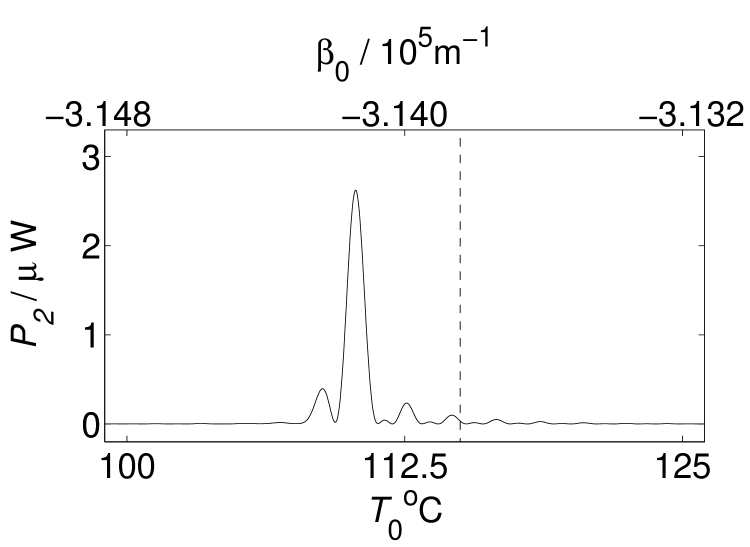
Figure 7: SHG tuning curve for periodic QPM crystal with a temperature profile varying according to Eq. (27). The parameters are: $L=5c\mbox{m}$, $t_{0}=1000^{\circ}$C/m, $D=0.5$, $r_{1}=0.95$, $r_{2}=0.75$, $\Lambda=10\mu\mbox{m}$, and $\lambda_{p}=1.6\mu\mbox{m}$. The dashed vertical line indicates the location of the maximum with $B(z)=0$.

Besides the fact that we have used a longer crystal, the simulation has been done with exactly the same numbers as used in the previous sections including the mirror losses. The only difference is that we have now scanned through the reference temperature $T_{0}$, with step-length $\Delta T_{0}=0.04^{\circ}\mbox{C}$, instead of through the pump wavelength which we have fixed at $\lambda_{p}=1.6\mu$m. With no temperature profile, the sample is phase matched at $|\beta_{0}|=\pi/\Lambda$ which is reached at $T_{0}\approx 115^{\circ}\mbox{C}$. The presence of a temperature profile changes the phase matching condition and we observe that the tuning curve on Fig. 7 is no longer sinc-shaped and that the main peak is shifted towards a higher absolute value of $\beta_{0}$. As we would expect from Eq. (15), we also observe that the maximum measured powers are around 25 times higher than the maximum powers measured in the experiments on the 1$c\mbox{m}$ long crystal in the last section.

In Fig. 8 we have plotted the retrieved temperature profile found from Fig. 7 via Eq. (23) together with the retrieved profile from a numerical experiment with $t_{0}=500^{\circ}$C/m.

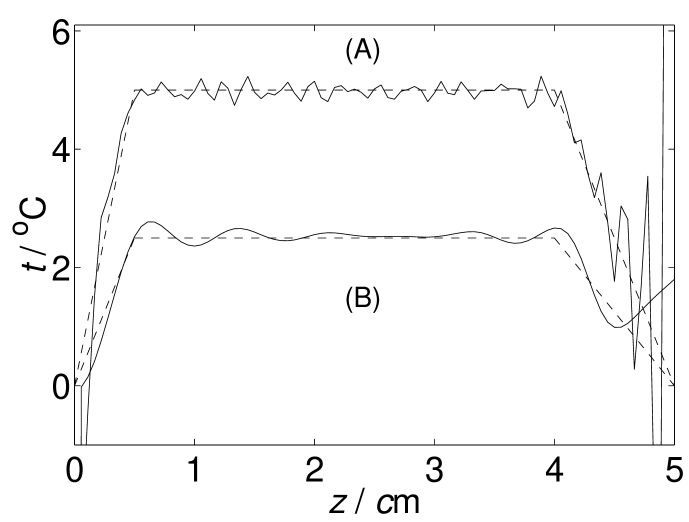
Figure 8: Retrieved temperature profiles for two different $t_{0}$: (A) $t_{0}=1000^{\circ}\mbox{C/m}$ and (B) $t_{0}=500^{\circ}\mbox{C/m}$. The full curves are the retrieved profiles and the dashed curves are the actual profiles used in the numerical experiments.

We see that we have excellent agreement between the actual profile and the retrieved profile and that the agreement seems to be better for the $t_{0}=1000^{\circ}\mbox{C/m}$ simulations. This is because we have used a larger reference temperature interval, $T_{0}\in[30^{\circ}\mbox{C}\;205^{\circ}\mbox{C}]$, for the $t_{0}=1000^{\circ}\mbox{C/m}$ curve than for the $t_{0}=500^{\circ}\mbox{C/m}$ curve for which $T_{0}\in[100^{\circ}\mbox{C}\;125^{\circ}\mbox{C}]$. We have used the larger interval to illustrate that $B(z)$ can in fact be assumed independent of $\beta_{0}$ over a considerable interval. The large oscillatory behavior just before $z=5c\mbox{m}$ is a result of the cut-off on the SH power measurement, i.e. the oscillations are not present if we lower the cut-off. $t(z)$ will of course not remain independent of the reference temperature over an interval this large. To illustrate that we still gain information with a narrower interval we show the $t_{0}=500^{\circ}\mbox{C/m}$ simulation. For longer crystals the tuning curves will in general be even narrower.

We remark that temperature profiles like the ones depicted in Fig. 8 have been determined before from experimental measurements on uniform lithium niobateschiek98nlgw . However, those experiments relied on the oven producing an even temperature profile, i.e. the absolute values of the linear increase and decrease at the beginning and at the end of the oven, respectively, were the same. The profiles from Fig. 8 are odd and hence cannot be determined through Fourier analysis without either aquiring phase information or, as we have done here, by utilizing the mirror setup.

VI Conclusion

In summary we have investigated how the mirror-setup paves the way for characterization of grating functions and temperature profiles via second-harmonic-power measurements only, i.e. without additional phase information. The grating function and temperature profile both become even functions in the propagation coordinate because of the mirror and we derived the Fourier scheme, including losses and phase shifts due to the mirror, to solve the inverse problem, i.e. to find the grating function and temperature profile knowing only the second harmonic tuning curve as a function of either wavelength or temperature. We verified the scheme through numerical simulations on bulk PPLN and showed how to retrieve information which is bandwidth limited to within the realizable phase-mismatch interval. In particular we investigated the case of the perfectly periodic duty-cycle waveguide for which we can determine both the domain length and the duty-cycle by simply looking at the tuning curve resulting from the mirror setup. Concerning temperature profiles we found that if we know the grating function then in theory we can determine any temperature profile. In particular we investigated the often encountered step-profile and we saw how this was beautifully retrieved.

References

- (1) R. L. Byer, “Quasi-phase Matched Nonlinear Interactions and Devices,” J. Nonlinear Opt. Phys. 6, 549–592 (1997).
- (2) M. M. Fejer, in Beam Shaping and Control with Nonlinear Optics, F. Kajzar and R. Reinisch, eds., (Plenum Press, New York, 1998), pp. 375–406.
- (3) J. Webjörn, V. Pruneri, P. Russel, J. R. M. Barr, and D. C. Hanna, “Quasi-phase-matched blue light generation with lithium niobate, electrically poled via liquid electrodes,” Electron. Lett. 30, 894–895 (1994).
- (4) K. El Hadi, M. Sundheimer, P. Aschieri, P. Baldi, M. P. De Micheli, and D. B. Ostrowsky, “Quasi-phase-matched parametric interactions in proton-exchanged lithium niobate waveguides,” J. Opt. Soc. Am. B14, 3197–3203 (1997).
- (5) P. Baldi, M. P. De Micheli, K. E. Hadi, S. Nouh, A. C. Cino, P. Aschieri, and D. B. Ostrowsky, “Proton exchanged waveguides in LiNbO3 and LiTaO3 for integrated lasers and nonlinear frequency converters,” Opt. Eng. 37, 1193–1202 (1998).
- (6) M. M. Fejer, G. A. Magel, D. H. Jundt, and R. L. Byer, “Quasi-Phase-Matched Second Harmonic Generation: Tuning and Tolerances,” IEEE J. Quantum Electron. 28, 2631–2654 (1992).
- (7) M. A. Arbore, A. Galvanauskas, D. Harter, M. H. Chou, and M. M. Fejer, “Engineerable compression of ultrashort pulses by use of second-harmonic generation in chirped-period-poled lithium niobate,” Opt. Lett. 22, 1341–1343 (1997).
- (8) K. Mizuuchi and K. Yamamoto, “Waveguide second-harmonic generation device with broadened flat quasi-phase-matching response by use of a grating structure with located phase shifts,” Opt. Lett. 23, 1880–1882 (1998).
- (9) S. Zhu, Y. Zhu, Y. Qin, H. Wang, C. Ge, and N. Ming, “Experimental Realization of Second Harmonic Generation in a Fibonacci Optical Superlattice of LiTaO3,” Phys. Rev. Lett. 78, 2752–2755 (1997).
- (10) P. Baldi, C. G. Treviño-Palacios, G. I. Stegeman, M. P. De Micheli, D. B. Ostrowsky, D. Delacourt, and M. Papuchon, “Simultaneous generation of red, green and blue light in room temperature periodically poled lithium niobate waveguides using single source,” Electron. Lett. 31, 1350–1351 (1995).
- (11) M. Cha, “Cascaded phase shift and intensity modulation in aperiodic quasi-phase-matched gratings,” Opt. Lett. 23, 250–252 (1998).
- (12) K. Gallo, G. Assanto, K. R. Parameswaran, and M. M. Fejer, “All-optical diode in a periodically poled lithium niobate waveguide,” Appl. Phys. Lett. 79, 314–316 (2001).
- (13) K. R. Parameswaran, M. Fujimura, M. H. Chou, and M. M. Fejer, “Low-Power All-Optical Gate Based on Sum Frequency Mixing in APE Waveguides in PPLN,” IEEE Photon. Technol. Lett. 12, 654–656 (2000).
- (14) L. Torner, C. B. Clausen, and M. M. Fejer, “Adiabatic shaping of quadratic solitons,” Opt. Lett. 23, 903–905 (1998).
- (15) S. Carrasco, J. P. Torres, L. Torner, and R. Schiek, “Engineerable generation of quadratic solitons in synthetic phase matching,” Opt. Lett. 25, 1273–1275 (2000).
- (16) S. K. Johansen, S. Carrasco, L. Torner, and O. Bang, “Engineering of spatial solitons in two-period QPM structures,” Opt. Commun. 203, 393–402 (2002).
- (17) G. Imeshev, M. Proctor, and M. M. Fejer, “Lateral patterning of nonlinear frequency conversion with transversely varying quasi-phase-matching gratings,” Opt. Lett. 23, 673–675 (1998).
- (18) P. E. Powers, T. J. Kulp, and S. E. Bisson, “Continuous tuning of a continuous-wave periodically poled lithium niobate optical parametric oscillator by use of a fan-out grating design,” Opt. Lett. 23, 159–162 (1998).
- (19) C. B. Clausen and L. Torner, “Self-Bouncing of Quadratic Solitons,” Phys. Rev. Lett. 81, 790–793 (1998).
- (20) C. B. Clausen and L. Torner, “Spatial switching of quadratic solitons in engineered quasi-phase-matched structures,” Opt. Lett. 24, 7–9 (1999).
- (21) L. Chanvillard, P. Aschiéri, P. Baldi, D. B. Ostrowsky, M. de Micheli, L. Huang, and D. J. Bamford, “Soft proton exchange on periodically poled LiNbO3: A simple waveguide fabrication process for highly efficient nonlinear interactions,” Appl. Phys. Lett. 76, 1089–1091 (2000).
- (22) R. Schiek, M. L. Sundheimer, D. Y. Kim, Y. Baek, G. I. Stegeman, H. Seibert, and W. Sohler, “Direct measurement of cascaded nonlinearity in lithium niobate channel waveguides,” Opt. Lett. 19, 1949–1951 (1994).
- (23) D. H. Jundt, “Temperature-dependent Sellmeier equation for the index of refraction, , in congruent lithium niobate,” Opt. Lett. 22, 1553–1555 (1997).
- (24) R. Schiek, H. Fang, and C. G. Treviño-Palacios, “Measurement of the non-uniformity of the wave-vector mismatch in waveguides for second-harmonic generation,” In Nonlinear Guided Waves and Their Applications Topical Meeting, OSA Technical Digest, pp. 256–258, paper NFA5–1 (Optical Society of America, Washington DC, 1998).
- (25) J. A. Armstrong, N. Bloembergen, and P. Pershan, “Interaction Between Light Waves in a Nonlinear Dielectric,” Phys. Rev. 127, 1918 (1962).