Basin structure in the two-dimensional dissipative circle map

Abstract

Fractal basin structure in the two-dimensional dissipative circle map is examined in detail. Numerically obtained basin appears to be riddling in the parameter region where two periodic orbits co-exist near a boundary crisis, but it is shown to consist of layers of thin bands.

1 Introduction

The circle map is one of the model systems that have been studied extensively in connection with the chaotic dynamics[1]. It represents dynamics of various types of physical systems with oscillatory motion under some external action, such as a kicked rotator, a bouncing ball [2, 3], Josephson junctions in microwave[4, 5], etc. Depending upon the strength and frequency of external field, it shows both quasi-periodic and mode-locked motions; Arnol’d tongue is a famous pattern that appears in the bifurcation diagram for these behaviors.

Recently, the present authors showed that this map has peculiar basin structure in the parameter region where two periodic orbits co-exist near a boundary crisis[6]. Numerically obtained basin appears to consist of a lot of dots and looks almost like a riddled basin, i.e. the basin that is a closed set without interior, yet with finite measure.

The riddled basin has been shown to appear for a chaos attractor that is confined within a subspace of the phase space[7, 8], but in the case of periodic attractor, there exists a finite trapping region, therefore, the basin should be an open set and cannot be a riddled basin.

The riddled-like structure in this case has been found to come from long transient chaotic motion and very small stability window for the periodic attractor within the transient chaotic “attractor”[6].

In this paper, we investigate in detail this riddled-like basin structure in the two-dimensional dissipative circle map, and show the basin actually consists of a lot of thin bands in spite of the appearance of the numerically obtained basin.

2 Two-dimensional circle map and riddled-like basin

The two-dimensional dissipative circle map is the map for the two variables $\theta$ and $r$,

$$\theta_{n+1} = \theta_{n}+\Omega-\frac{K}{2\pi}\sin(2\pi\theta_{n})+br_{n}\quad\mbox{mod 1},$$ (1)

$$r_{n+1} = br_{n}-\frac{K}{2\pi}\sin(2\pi\theta_{n}),$$ (2)

where $\Omega$, $K$, and $b$ are parameters, and the dynamics is dissipative when $b<1$. This map is equivalent with the bounce map that describes the motion of bouncing ball on a vibrating platform within the high bounce approximation[9]; The basin structure of the bounce map was shown to be completely scattered and appear almost riddling[6].

As for the 2-d circle map, the basin becomes riddled-like for $K=6$, $\Omega=0.03138$, and $b=0.1$; With these parameters, there co-exist two periodic attractors, namely, the period two and the period four attractors. In Fig.1, we show the basin structure of the period four attractor by plotting dots at the points within the basin out of $2000\times 2000$ grid points in the phase space, i.e. for each gid points, we examine the orbits, and if the orbit ends up in the the period four attractor, a dot is plotted at the point where we started, but if the orbit ends up in the period two attractor, the point is left blank. We see a very much riddled-like basin although it cannot be a riddled-basin in the mathematical definition[6, 7, 8].

In the following, we investigate the detailed structure of such a basin.

3 One-dimensional circle map

First, we explore the case of $b=0$, then the variable $r$ becomes irrelevant for the dynamics, and eq.(1) reduces to the one-dimensional circle map

$$\theta_{n+1} = f(\theta_{n})$$ (3)

$$= \theta_{n}+\Omega-\frac{K}{2\pi}\sin(2\pi\theta_{n})\quad\mbox{mod 1}.$$

It is well known that, for $|K|<1$, one finds the Arnol’d tongues where the motion is mode locked, and this becomes the complete devil’s staircase at $|K|=1$, then chaotic and non-chaotic regions are densely interwoven in the parameter space for $|K|>1$; the last region is the one we will look at carefully.

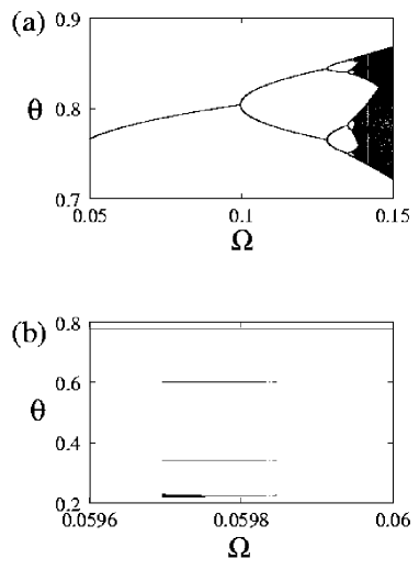
Figure 2: Bifurcation Diagram for $b=0$ in the two-dimensional circle map upon changing $\Omega$ with $K=6$.

Two periodic attractors can co-exist in some parameter regions for $|K|>1$. The bifurcation diagram is displayed in Fig.2(a) upon changing $\Omega$ with $K=6$. It shows the period doubling and chaos as increasing $\Omega$. If we blow up the parameter region $0.0596<\Omega<0.06$ (Fig.2(b)), we can see another periodic attractor appears around $\Omega=0.0598$. In this parameter region, the period one attractor is stable, whereas a new period three attractor appears and bifurcates into the period six as decreasing $\Omega$. Upon decreasing $\Omega$ further, this attractor bifurcates into a chaos attractor, then it is destroyed suddenly through a boundary crisis of the period one basin.

In the 1-d map, the co-existence of the two periodic orbits can be seen easily by considering the $n$’th iterates of eq.(3), i.e. $f^{n}(\theta)$. The period $n$ attractor $\theta_{i}$ ($1\leq i\leq n$) is given by

$$\theta_{i}=f^{n}(\theta_{i}).$$ (4)

The function $f^{1}(\theta)$ and $f^{3}(\theta)$ are plotted in Fig.3 for $K=6$ and $\Omega=0.0598$. We see that the both of $f^{1}(\theta)$ and $f^{3}(\theta)$ have the stable solution of eq.(4), which shows eq.(3) has both the period one and the period three attractor at this parameter. The absolute value of the slope of $f^{3}(\theta)$ is much larger than 1 for most of the value of $\theta$, which implies that the period three attractor is stabilized only for a very small parameter region.

Another consequence that comes from the steepness of $f^{3}(\theta)$ is the fact that the period three attractor has an extremely small trapping region, i.e. a connected region that any orbit inside converges to the attractor without leaving the region. The basin can be constructed as the union of its pre-iterates, and the fact that $f^{3}(\theta)$ consists of a lot of nearly vertical lines means that the pre-iterates are even smaller than their images and scattered all over the $\theta$-axis, therefore, the basin structures of these attractors are scattered and mixed each other.

We measure the uncertainty exponent[10], or the final state sensitivity $\alpha$, which is defined as the exponent for the probability $f_{d}(\epsilon)$ that two points separated from each other by small distance $\epsilon$ in the phase space are in different basins;

$$f_{d}(\epsilon)\sim\epsilon^{\alpha}.$$ (5)

If $\alpha$ is small, the final state is difficult to predict from the initial state, which means the two basins are intricate. For $K=6$ and $\Omega=0.0598$, the estimated value of the uncertainty exponent is $\alpha=6\times 10^{-2}$. This means that the fractal dimension of the basin boundary is close to 1, or the dimension of the phase space $d$, because the fractal dimension $d_{f}$ is related to $\alpha$ through[10]

$$d_{f}=d-\alpha.$$ (6)

It is conceivable that, for large $n$, $f^{n}(\theta)$ consists of lines that are nearly vertical, thus if the period $n$ attractor is stable for large $n$ and coexists with another periodic attractor, the uncertainty exponent should be close to $0$. Note that the parameter region of such co-existence is extremely small in general.

4 Two-dimensional circle map

4.1 the $b=0$ case

We consider the basin structure for the $b=0$ case in the full two-dimensional phase space of the circle map (1) and (2), although the map is essentially one-dimensional in this case; eq.(1) becomes eq.(3), and the variable $r$ simply follows $\theta$ through eq.(2). We discuss its basin structure in the full phase space for $K=6$ and $\Omega=0.0598$, where the period one and the period three attractors co-exist.

From eq.(2), the trajectory in the phase space is on the line

$$r_{n+1}=-\frac{K}{2\pi}\sin(2\pi\theta_{n}).$$ (7)

Namely, $r_{n+1}$ is determined only by $\theta_{n}$, which means that the point $(\theta_{n},r_{n})$ moves along the line (7) while the system shows the transient chaos. After some iterations, $(\theta_{n},r_{n})$ eventually falls into the trapping region of either the period one or the period three attractor on the line. Figure 4 shows the “attractor” of the transient chaos with the period one and the period three attractor for $K=6$, $\Omega=0.0598$, and $b=0$, where the transient chaos attractor is simply a line.

It is easy to understand that the basin is made of a lot of vertical bands as shown in Fig.5(a), because the variable $r$ does not affect the dynamics. The examined grid points are the same as the one in Fig.1, and the grid points that end up in the period three attractor are marked by black dots, whereas the points that lead to the period one attractor are left blank. We may not see the bands thinner than the grid spacing; The finer grid we use, the more thin bands show up. The ratio, however, of black dots to all the grid points examined does not change significantly.

4.2 the $0\mathrel{\mathchoice{\lower 2.58334pt\vbox{\halign{$\m@th\displaystyle\hfil#\hfil$\cr<\crcr\sim\crcr}}}{\lower 2.58334pt\vbox{\halign{$\m@th\textstyle\hfil#\hfil$\cr<\crcr\sim\crcr}}}{\lower 2.58334pt\vbox{\halign{$\m@th\scriptstyle\hfil#\hfil$\cr<\crcr\sim\crcr}}}{\lower 2.58334pt\vbox{\halign{$\m@th\scriptscriptstyle\hfil#\hfil$\cr<\crcr\sim\crcr}}}}b\ll 1$ case

The vertical band basin structure for the $b=0$ case will be modified when $b\neq 0$. Fig.5(b) shows the basin of the period three attractor for the very small value of $b=10^{-5}$ with the same $\Omega$ and $K$ as in Fig.5(a). In Fig.5(b), the basin seems to be made of a lot of dots in addition to some vertical bands. We believe, however, the dotted structure is numerical artifact: the vertical stripes for $b=0$ should be deformed only slightly to be the diagonal stripes for such a small $b$.

In the following, we examine the procedure to construct the basin of the period three attractor for $b\ll 1$ to convince ourselves that it has a layered structure.

Let us start by noting that, from eq.(1), the point that will be mapped at $\theta_{n+1}=\theta^{*}$ with the arbitrary $r_{n+1}$ at ($n+1$)’th step is on the line

$$r_{n}=-\frac{1}{b}\left(\theta_{n}+\Omega-\frac{K}{2\pi}\sin(2\pi\theta_{n})-\theta^{*}\right)$$ (8)

at the $n$’th step.

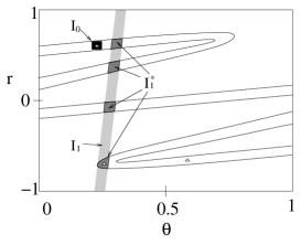
Figure 6: The schematic construction of the basin for the period three attractor for $b\ll 1$. The white band represents the transient chaos “attractor” given by eq.(7) with the width $b$. The region $I_{0}$ (black square) is the $\ell\times b$ ($\ell<b$) region within the trapping region of the attractor. The region $I_{1}$ is the pre-iterate of $I_{0}$ and it extends along the line (8). The most of of the pre-iterate of $I_{1}$, or $I_{2}$, goes out of the range shown in the graph; Only the region $I^{*}_{1}$, the parts within the band, remain in the graph.

The trapping region of the period three attractor has a very narrow width in the $\theta$-direction, but should be elongated in the $r$-direction for $b\ll 1$. Suppose $I_{0}$ is a part of the trapping region with the size $\ell\times b$, where $\ell$ ($b$) is the length of the region in the $\theta$- ($r$-)direction and we take $\ell\leq b$ (Fig.6). The transient chaos “attractor” is now a band with the width $O(b)$ as we see from eq.(2). Let $I_{1}$ be the pre-iterate of $I_{0}$, then $I_{1}$ is stretched along the line (8). The width of $I_{1}$ in the $\theta$-direction is also $O(b)$ because of the relation

$$\theta_{n}=\theta_{n+1}-r_{n+1}-\Omega,$$ (9)

which we have from eqs. (1) and (2). The extension of $I_{1}$ along the $r$-direction is $O(1)$ because

$$r_{n}=\frac{1}{b}\left(r_{n+1}-\frac{K}{2\pi}\sin(2\pi\theta_{n})\right)$$ (10)

due to eq.(2).

Then, we now consider how $I_{2}$, i.e. the pre-iterate of $I_{1}$, is distributed. Let the part of $I_{1}$ along the line (7) with the width $b$ be $I^{*}_{1}$ (Fig.6). The most part of the pre-iterate of $I_{1}$, namely $I_{2}$, is outside of the $r\sim O(1)$ region when $b\ll 1$, and only the pre-iterate of the part $I^{*}_{1}$ stays in the region of $r\sim O(1)$. The region $I_{2}$ consists, in turn, of the bands (8) with the value $\theta^{*}$ of the corresponding part of $I^{*}_{1}$. Repeating the above procedure, we obtained the basin made of a lot of thin bands.

5 Numerical analysis

We now present numerical evidences of the band structure obtained in the above discussion, and estimate the distribution function of the band width.

In order to study the local basin structure around an arbitrary point $(\theta_{0},r_{0})$ that is in the period three basin, we examine the points along the circle with the radius $\epsilon$ centered at the point. The function $F(\phi;\epsilon)$ plotted in Fig.7 is the function that takes the value of 1 if the point on the circle at the angle $\phi$ around the central point $(\theta_{0},r_{0})$ is in the period three basin, and zero otherwise; the angle $\phi$ is measured from the $r$-direction. This function should take the value of 1 around $\phi\approx 0$ and $\pi$ if the central point $(\theta_{0},r_{0})$ is in the basin of a vertical thin band of the width smaller than $\epsilon$.

Figure 7 shows $F(\phi;\epsilon)$ for three different values of $\epsilon$ around the same point $(\theta_{0},r_{0})=(0.133,0.1)$ for the parameters $K=6$ and $\Omega=0.0598$ with the very small value of $b=10^{-5}$.

When $\epsilon=10^{-3}$, $F(\phi;\epsilon)$ looks random and hardly shows any signs of the layered structure (Fig.7(a)). About 5% of the points on the circle are in the period three basin. As for $\epsilon=10^{-4}$, the band structure of the basin is beginning to show in the plateaus around $\phi\approx 0$ and $\pi$ (Fig.7(b)). For $\epsilon=10^{-5}$, $F(\phi;\epsilon)=1$ for all value of $\phi$ (Fig.7(c)). From these results, we can estimate the width of the basin $l$ at $(\theta_{0},r_{0})=(0.133,0.1)$ as $l\approx 5\times 10^{-5}$.

Repeating the above procedure for a lot of points of $(\theta_{0},r_{0})$, we can determine the probability $R(l)$ that a point in the period three basin is in the band whose width is smaller than $l$. This is related to the probability density $P(l)$ to pick a band of period three basin with the width $l$ by

$$R(l)=\int_{0}^{l}P(l^{\prime})dl^{\prime}.$$ (11)

Numerical results of $R(l)$ are shown in Fig.8 in the log-log plot for each basin of the three cases of $b=0$, $10^{-5}$, and $0.1$; the difference between $R(l)$ for $b=0$ and that for $b=10^{-5}$ are invisible. We see that $R(l)$’s are very flat over many decades of $l$, and if we fit the plots in Fig.8 by the straight lines, namely, the power

$$R(l)\propto l^{\beta},$$ (12)

with the exponent $\beta$, we obtain the same value of $\beta$ for the two competing basins, $\beta=0.06$ for both period one and period three basin in the case of $b=0$ and $10^{-5}$, and $\beta=0.03$ for both period two and period four basin in the case of $b=0.1$. For larger $b$, the exponent $\beta$ becomes large, which means there are more thin bands.

In principle, the exponents can be different for the two competing basins; $\beta_{1}$ for the basin 1 and $\beta_{2}$ for the basin 2. If $p_{n}$ is the probability that a phase point belongs to the basin $n$, then the probability $f_{d}(\epsilon)$ that two points separated from each other by small distance $\epsilon$ in the phase space are in different basins is given by

$$f_{d}(\epsilon)\sim p_{1}R_{1}(\epsilon)+p_{2}R_{2}(\epsilon)\sim\epsilon^{\beta_{1}}+\epsilon^{\beta_{2}}$$ (13)

for $\epsilon\ll 1$, where $R_{n}(\epsilon)$ is the probability that a point in the basin $n$ is on the band whose width is narrower than $\epsilon$. From the definition of $\alpha$ by (5), we have

$$\alpha=\min_{n}\beta_{n},$$ (14)

which is confirmed by estimating $\alpha$ independently, $\alpha=0.06$ for $b=0$ and $10^{-5}$ and 0.03 for $b=0.1$.

The two exponents $\beta_{1}$ and $\beta_{2}$ are same for all of our cases as mentioned above. There are, however, no geometrical reasons that impose the equality, therefore, this should come from the mechanism that the basin structure is generated, namely, the basins are mixed through stretching and folding by a transient chaos, but the detailed analysis remains to be done.

6 Summary and discussions

From the analysis of the map and the numerical evidences, we have concluded that the basins for the periodic attractors have the layered band structure in the circle map for the parameter region where the two periodic attractors co-exist. This is quite different from the impression one might have from the numerically obtained basin (Fig.1). Even a small value of $b$ like $10^{-5}$ changes the appearance of the basin rather drastically from the obvious layered structure in the $b=0$ case (Fig.5).

By examining a neighboring region of each point, we have estimated the distribution of the band width of the basin, and shown that the distribution is hardly changed by the small value of $b=10^{-5}$ (Fig.8); this is quite a contrast with the change in the basin appearance mentioned above.

This apparent paradox is resolved when we plot the basin with the slightly slanted grid for the case of $b=0$ and find the result is nearly the same with that for $b=10^{-5}$ (Figs.5(b) and 9). In the case of $b=0$, the basin must consist of vertical bands, but if the basin is examined numerically on the slanted grid points, the dotted structure is obtained. This is because the numerous thin bands that escape from the straight grid points graze through the slanted grid points.

The Lyapunov graph of the circle map has been studied in the literature and shown the structure is intricate especially for the region of large $K$[1, 11]. This should come from the intricate basin structure studied here; If one try to plot the Lyapunov graph with only one set of initial values for the variable, one would get an intricate structure upon changing the parameters of the map as they go through the region where the basin structure is intricate. This is because the basin that the fixed initial point belongs to changes wildly even if the global change of the basin structure is minute. In these regions, the system shows multi stability and the Lyapunov exponents that correspond to two or more attractors are chosen almost randomly in the graph.

The basin structure in the similar situation has been studied by Dronov and Ott[12]. They studied the case where the riddled basin is destroyed by the de-stabilization of chaos attractor due to a periodic orbit, and they found “stalactite structure” of basin. There are some similarities in the mechanism to our case, and their stalactite basin may be compared with our layered band structure of basin, but the major difference is that, in their case, the chaos attractor is confined in a subspace of the phase space as is necessary to have a riddled basin while the chaos is embedded in the full phase space in our case.

In summary, we investigated the basin structure of the two-dimensional circle map. From the analysis in the $b\ll 1$ case, in the parameter region where the period $m$ attractor coexists with the period $n$ attractor, the basin structure is apparently riddled-like, but is made of a lot of thin bands.

Figure 1: The riddled-like basin of the period four attractor (dots) for the two-dimensional circle map with $K=6,\Omega=0.03138$ and $b=0.1$.

Figure 3: The profile of $f(\theta)$ (a), and $f^{3}(\theta)$ (b) for $K=6$ and $\Omega=0.0598$ . The dotted lines show $f(\theta)=\theta$. The attractor of the period one ($\Box$) and the period three ($\triangle$) are also indicated.

Figure 4: The period three attractor ($\triangle$) and the period one attractor ($\Box$) with the temporal attractor of the transient chaos (dots) for $K=6,\Omega=0.0598$, and $b=0$.

Figure 5: The numerically obtained basin of the period three attractor (dots) for $K=6,\Omega=0.0598$ for $b=0$ (a) and $b=10^{-5}$ (b). The straight grid points of $2000\times 2000$ are examined.

Figure 7: The function $F(\phi;\epsilon)$ around the point $(\theta_{0},r_{0})=(0.133,0.1)$, which is in the period three basin, with $K=6$, $\Omega=0.0598$, and $b=10^{-5}$ for $\epsilon=10^{-3}$ (a), $10^{-4}$ (b), and $10^{-5}$ (c).

Figure 8: The probability $R(l)$ that the band width is smaller than $l$ for each basin for $K=6$, $\Omega=0.0598$, and $b=0$ (a), $10^{-5}$ (b), and for $K=6$, $\Omega=0.03138$, and $b=0.1$ (c); ($\diamond$) for a majority basin (the period one or period two basin) and ($+$) for a minority basin (the period three or period four basin). The dotted and dashed lines represent the lines of $l^{\beta}$ with $\beta=0.06$ for $b=0$ and $10^{-5}$, and $\beta=0.03$ for $b=0.1$

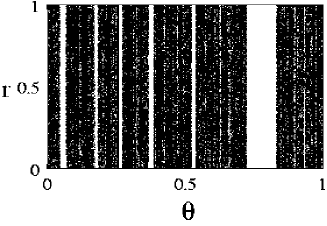
Figure 9: The numerically obtained basin structure for $b=0$ using the slanted grids for $b=0$. The other parameters are same as in Fig.5(a).

References

- [1] H.G. Schuster: “Deterministic Chaos”, (VCH, Germany, 1989).
- [2] R. M. Everson: Physica D 19 (1986) 355.
- [3] G. A. Luna-Acosta: Phys. Rev. A 42 (1990) 7155.
- [4] T. Bohr, P. Bak, and M.H. Jensen: Phys. Rev. A 30 (1984) 1970.
- [5] S. Habip, M. Bauer, D. -R. He and W Martienssen: Physica D 59, (1992) 378.
- [6] S. Fukano, Y. Hayase and H. Nakanishi: J. Phys. Soc. Jpn., 71 (2002) 2075.
- [7] A. S. Pikovsky and P. Grassberger: J. Phys. A 24 (1991) 4587.
- [8] E. Ott, J. C. Alexander, I. Kan, J. C. Sommerer and J. A. Yorke: Physica D 76 (1994) 384.
- [9] The bounce map given by eq.(1) of ref. References) reduces to the 2-d circle map by the replacement, , , , , .
- [10] A. J. Lichtenberg and M. A. Lieberman: “Regular and Chaotic Dynamics”, (Springer-Verlag, New York, 1992).
- [11] J.C. Bastos de Figueiredo and C.P. Malta: Int. J. Bifur. Chaos, 8 (1998) 281.
- [12] V. Dronov and E. Ott: Chaos, 10 (2000) 291.