Multiple Timescale Dynamics in Economic Production Networks

Abstract

We describe a new complex system model of an evolving production economy. This model is the simplest we can envisage which incorporates the new observation that the rate of an economic production process depends only on the minimum of its supplies of inputs. We describe how this condition gives rise to a new type of complex multiple timescale dynamical evolution through a novel type of bifurcation we call a trapping bifurcation, which is also shown to be one cause of non-equilibrium economic behaviour. Such dynamics is an example of meta-level coupling which may also arise in other fields such as cellular organization as a network of molecular machines.

Introduction. Recently physicists have been devoting a great deal of attention to economic and financial phenomenamant . Economic dynamics is easily observed to be far from equilibrium where periodic recessions, unemployment and unstable prices occur persistently. An understanding of the origins of this behaviour from the viewpoint of complex dynamical systems theory would be very valuable. Our modelphysA , which we hope takes a step in this direction, is based on von-Neumann’svmpap-vmbook neoclassical model of economic production and catalytic chemical reaction network dynamicskan .

The original von Neumann model (VNM) of economic production assumes that each good is produced jointly with certain others, in an analogous way to a chemical reaction. A production process is the operation which converts one bundle of goods, including capital equipment, into another bundle of goods, including the capital equipment. Capital goods therefore function approximately like catalysts in chemical reactions, reformed at the end of the reaction in amounts conserved in the reaction. Consumption of goods is assumed to take place only through production processes, including life necessities consumed by workers, and all income is reinvested in production. Therefore the VNM is defined by a fixed input matrix and a fixed output matrix, representing, the fixed stochiometric ratios of input products and output products for each process. An example of such an economic network is shown in Fig.1. Each process is assumed to have unit time duration, longer processes being broken down into several processes with intermediate products. The VNM is defined as a static equilibrium model describing relationships between the variables which must hold at equilibrium. Equilibrium is a state of ‘balanced growth’ where prices are constant. There are no dynamics defined by the model which might describe out of equilibrium or approach to equilibrium behaviour.

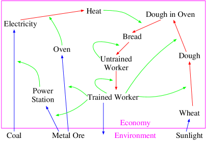
Figure 1: An Economy. Red lines are production flows, blue lines flows to and from the environment (including other countries) and green lines are catalytic effects. Some processes are autocatalytic.

However it is rarely the case that economic processes are in equilibrium. For example consider a simple bakery with input: (dough, baker, oven) and output: (bread, baker, oven), so that the baker and the oven are catalysts. We observe that the rate of bread production, and economic processes in general, depends on the quantity of the minimum of its input supplies and not on the quantities of its other supplies. I.e. the baker working at full pace can only fill ovens at a certain rate. Similarly employing more bakers will not increase bread production if the ovens are already full. This is in direct contrast with a chemical reaction obeying the law of mass action, where an increase in concentration of any of its input species will increase the rate of reaction.

This minimum condition leads directly to multiple timescalesfuj . Consider a factory assembling bicycles from wheels and frames at a given rate. Suppose for some reason the rate of supply of wheels increases so that their price drops. To maximise efficiency the factory will try to use all its funds to expand production, buying the extra wheels and demanding more frames. A factory with large funds may demand frames so strongly that the the frame-makers respond to it and increase their supply rate. In this way the wheel-makers and frame-makers production rates may become synchronised. A factory with small funds on the other hand may only weakly influence the frame supply rate. Its bicycle production rate will be determined by the supply rate of whichever is the most expensive, and may switch between the rates as price levels change. The factory will have inefficient periods with surpluses of frames or wheels, but to avoid this by not using all its funds would still not be maximally efficient.

Here we show how such multiple timescales arise ‘endogenously’ in a new model of an economy of coupled processes which is different from the VNM in that we explicitly take into account the way a process’ production rate depends on the minimum of its input supplies.

Model. Although our model ignores many details, we believe it captures the essential characteristics of a evolving production-marketing network, in the simplest way possible. The system is defined by a fixed number of processes $K_{I}$ and products $K_{J}$ with input stochiometric ratios $a_{ij}$ and ouput stochiometric ratios $b_{ij}$, where $i$ labels the processes and $j$ the products. Each process has supplies of its products $S_{ij}(t)$, it also has a dynamical fitness called funds $F_{i}(t)$, measured in dollars, which represents the ‘size’ or ‘intensity’ of the process. The model can be conveniently broken down into four simple parts.

(i) Processing. Here all processes simultaneously manufacture goods so that their supplies after processing, denoted with ‘^∗’, are given by,

$$S^{*}_{ij}(t)=S_{ij}(t)+(b_{ij}-a_{ij})Min_{k}(S_{ik}(t)/a_{ik})$$ (1)

where the processing rate is given by $Min_{k}(S_{ik}(t)/a_{ik})$ where $Min_{k}(x_{k})$ denotes the minimum over $x_{k}$.

(ii) Product revaluation. The value, or price $p_{j}(t)$, of a product is recalculated after processing and depends on the overall supply available in the whole economy and on how much all the processes want it. To measure how much the processes want the product we consider how much they will pay for it and each process therefore divides its funds $F_{i}(t)$ into demands $D_{ij}(t)$ for its input products. The new product value $p_{j}(t)$ is then given by

$$p_{j}(t)=\frac{Total\hskip 2.84544ptDemand}{Total\hskip 2.84544ptSupply}=\frac{\sum_{i}D_{ij}(t)+D^{e}_{j}}{\sum_{i}S^{*}_{ij}(t)+S^{e}_{j}},$$ (2)

where $S^{e}_{j}$ and $D^{e}_{j}$ are possible external supplies and demands coming from, say, another country.

There are many ways a process may allocate its funds into demands. If we consider a feedback from the price the funds should be divided according to $a_{ij}p_{j}(t-1)$ since this is process $i$’s best estimate of the per unit cost of input $j$ depending on the most recent known price $p_{j}(t-1)$. Alternatively the process may simply divide its funds according to the ratios $a_{ij}$. Here we will consider,

$$D_{ij}(t)=F_{i}(t)(\gamma\frac{a_{ij}p_{j}(t-1)}{\sum_{j}a_{ij}p_{j}(t-1)}+(1-\gamma)a_{ij})$$ (3)

where the parameter $0<\gamma<1$ quantifies the feedback from the price. In fact we will show that the interesting behaviour is found independently of $\gamma$, the important points being $D_{ij}(t)\propto F_{i}(t)$ $\forall j$ and $\sum_{j}D_{ij}(t)=F_{i}(t)$.

(iii) Product resharing. Processes obtain new supplies for processing simply according to

$$S_{ij}(t+1)=D_{ij}(t)/p_{j}(t)$$ (4)

so that processes with relatively large funds obtain larger proportions of the available supply.

(iv) Process revaluation. The new process funds are,

$$F_{i}(t+1)=\sum_{j}S^{*}_{ij}(t)p_{j}(t)$$ (5)

so that processes with larger manufactured supplies obtain greater proportions of the available funds, and in this way the system becomes an evolving network.

Results. These equations have the novel property that they switch their form depending on which product is the minimum at any time. Synergetic effects then appear because the dynamics itself selects the equations which determine its own future evolution. We will show that this strong non-linearity leads to the new type of very complex multi-timescale dynamics illustrated in Fig.2, focusing on $\gamma=0$ since the analysis is much simpler.

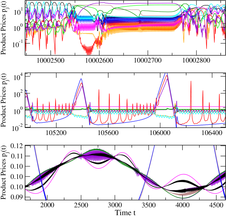
Figure 2: Three examples of multi-timescale time series produced from 15 process, 10 product networks, ($\gamma=0.9$).

We first show that even the simplest single process, in a fixed environment, will, under general conditions, oscillate periodically due to a novel switching mechanism and furthermore this has interesting economic relevance.

This $K_{I}=1$, $K_{J}=3$ system has one input product I, one catalyst C, and one output product O, reacting with non-zero stochiometric ratios $a_{I}=a_{C}=b_{C}=b_{O}=1/2$ with $\gamma=0$. It has 3 variables, its input supplies $S_{I}(t)$, catalyst supplies $S_{C}(t)$ and funds $F(t)$, where we drop the process label $i$. There are two phases: (X) excess input, $S_{I}(t)>S_{C}(t)$ and (Y) excess catalyst, $S_{I}(t)<S_{C}(t)$, such that Eq.4, $S_{I}(t+1)=1/2F(t)/p_{I}(t)$ and $S_{C}(t+1)=1/2F(t)/p_{C}(t)$ becomes,

$$(X)\hskip 14.22636ptS_{I}(t+1)=\frac{1/2F(t)(S_{I}(t)-S_{C}(t)+S^{e}_{I})}{1/2F(t)+D^{e}_{I}}$$ (6)

$$(Y)\hskip 14.22636ptS_{I}(t+1)=\frac{1/2F(t)S^{e}_{I}}{1/2F(t)+D^{e}_{I}}$$ (7)

$$(X,Y)\hskip 14.22636ptS_{C}(t+1)=\frac{1/2F(t)(S_{C}(t)+S^{e}_{C})}{1/2F(t)+D^{e}_{C}}$$ (8)

where we have omitted the (X) and (Y) $F(t)$ equations for simplicity and where $S^{e}_{I},S^{e}_{C},S^{e}_{O}$ and $D^{e}_{I},D^{e}_{C},D^{e}_{O}$ are fixed external supplies and demands of the three products respectively. Here, since $\gamma=0$ and $a_{I}=a_{C}$, (X) and (Y) switch whenever the prices $p_{I}(t)$ and $p_{C}(t)$ cross.

To understand the novel dynamical features of this system it is sufficient to consider the interaction of the phase (X) and phase (Y) fixed points. Denoting these two fixed points by superscript ‘^x,y’ we find that, although the fixed point positions are different, the fixed point prices in both phases are the same and given by,

$$p_{I}^{x,y}=p_{O}^{x,y}=\frac{D^{e}_{I}+D^{e}_{O}}{S^{e}_{I}+S^{e}_{O}},\hskip 28.45274ptp_{C}^{x,y}=\frac{D^{e}_{C}}{S^{e}_{C}}.$$ (9)

Therefore a process in equilibrium acts to make its input and output product prices equaleffic . This interesting non-trivial relationship has the observable consequence that for example scaling both $D^{e}_{O}$ and $S^{e}_{O}$ by the same constant factor will change the price of both $O$ and $I$, although one would naively expect that such a scaling should leave the prices unchanged.zerofp

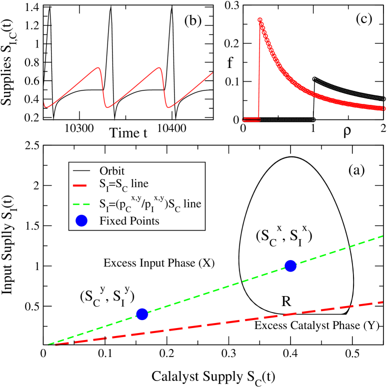
Figure 3: (a) The switching state; creation of periodic orbit from node and focus. The $S_{I}=S_{C}$ line (see key) divides the (X) and (Y) phases, whose fixed points are shown labelled. The fixed points are such that they lie on the $S_{I}=S_{C}(p_{C}^{x,y}/p_{I}^{x,y})$ line, (see key). Therefore only one can be compatible with its phase. Here, in the switching state shown, where $p_{C}^{x,y}/p_{I}^{x,y})>1$ the (X) fixed point is compatible since $S_{I}^{x}>S_{C}^{x}$, but the (Y) fixed point is incompatible since $S_{I}^{y}>S_{C}^{y}$. When the trajectory is in the (Y) phase it is attracted to the stable node $(S_{C}^{y},S_{I}^{y})$, which is incompatible with phase (Y). Therefore the phase boundary must be crossed and the system switches to an oscillation around the $(S_{C}^{x},S_{I}^{x})$ focus. This then causes the system to be reinjected into the (Y) phase again, producing the clockwise orbit. Furthermore, regardless of initial conditions, the system is always reinjected at the point $R$ thereby producing a limit cycle. Since $S_{I}^{y}=S_{C}^{x}$, the fixed points approach each other as $p_{C}^{x,y}/p_{I}^{x,y}$ approaches 1 from above and therefore the switching frequency increases while the amplitude decreases as confirmed in (c). (b) Time series of input supply $S_{I}(t)$ (black) and catalyst $S_{C}(t)$ (red) for a single process with $\gamma=1$. (c) Variation of switching frequency $f$ against $\rho=(p_{C}^{x,y}/p_{I}^{x,y})$ from Eq.9. $\gamma=0$ (black), $\gamma=1$ (red). As $\gamma$ increases the bifurcation point decreases and the frequency $f$ increases.

However as shown in Fig.3(a), which shows a typical time series variation in the $S_{I}(t)$, $S_{C}(t)$ plane, the process will not in general be at a fixed point, but oscillates periodically. Although neither phase (X) nor (Y) has a periodic attractor on its own, a limit cycle is created by a novel trapped switching mechanism which arises due to the minimum dynamics as explained in Fig.3(a). As shown the ratio of the fixed point values $\rho=(p_{C}^{x,y}/p_{I}^{x,y})$ acts as a trapping bifurcation parameter since when $\rho>1$ the switching state is obtained but when $\rho<1$ the system remains at the node without oscillating.

The switching state is plausible economically. In the switching state we find the fund fixed points are such that $F^{x}=\rho F^{y}>F^{y}$. Therefore when the system is in the excess catalyst phase (Y) its funds $F(t)$ decrease and it acts to reduce $S_{C}(t)$ (Eq.8). However the decrease in $S_{C}(t)$, since it is not the minimum supply, has no effect on the processing rate, and $S_{I}(t)$ (Eq.7) is therefore not affected by the change in $S_{C}(t)$. In the excess supply phase (X) on the other hand, the funds $F(t)$ increase and the process acts to increase $S_{C}(t)$ (Eq.8) which increases the processing rate and decreases $S_{I}(t)$ (Eq.6) producing the oscillation. Furthermore as explained in Fig.3(a)(c) the switching frequency decreases as $\rho$ increases. This is to be expected economically. The price fixed points are determined by the external environment. When $p_{C}^{x,y}>>p_{I}^{x,y}$ the process demands will have much less affect on $p_{C}(t)$ than $p_{I}(t)$. Therefore in the excess supply phase (X) $S_{C}(t)$, and therefore the processing rate, will only increase slowly and $S_{I}(t)$ will be reduced only slowly, producing large amplitude slow oscillations.

We therefore expect that even a single process in a fixed environment will have periodic dynamics, with periods of (X) full employment ($S_{I}(t)>S_{C}(t)$) interrupted by periods of (Y) unemployment, ($S_{I}(t)<S_{C}(t)$).

Through simulations we find Eqs.9 also seem to hold in the $\gamma>0$ case. The same switching state appears, see Fig.3(b)(c), but the exact bifurcation point varies. Furthermore the equivalence between switching and price crossing, seems to be still approximately true. However the switching dynamics is more complex as shown in Fig.3(b). This is interesting since one would naively expect that using price information should allow the process to obtain more balanced input supplies and processing to occur more smoothly. However doing so moves the process nearer the trapping birfurcation enhancing the switching feedback effects. This can produce quasiperiodic or weakly chaotic dynamics.

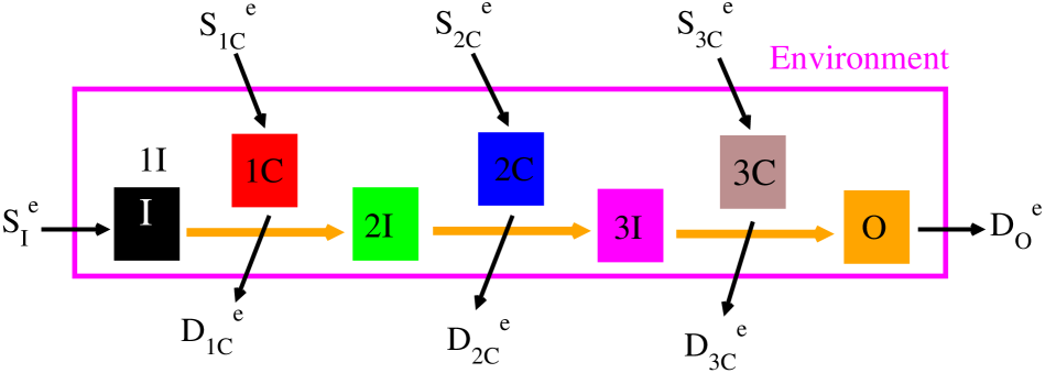
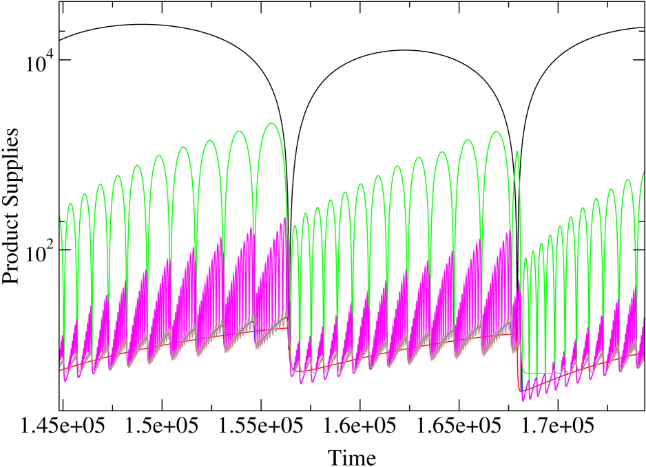
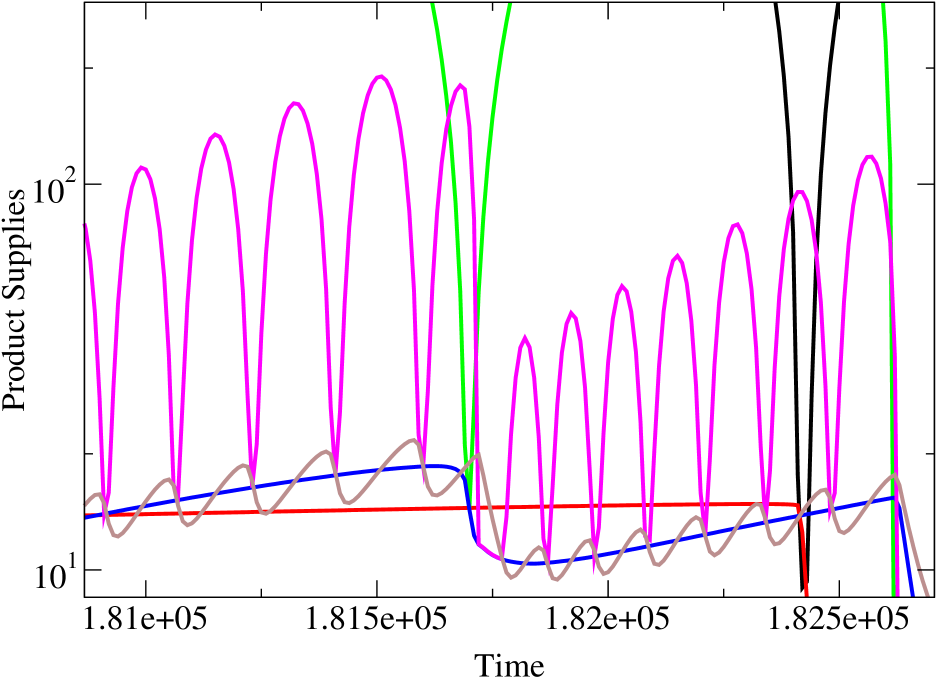
Figure 4: Hierarchical multiple timescale limit cycle attractor in process chain in fixed environment. (a) Diagram of a 3 process 7 product chain. 3 products are catalysts, one in each process each with a fixed external supply $S_{iC}^{e}$ and demand $D_{iC}^{e}$, defining an external price $p_{iC}^{x,y}=D_{1C}^{e}/S_{1C}^{e}$ for each catalyst. There is one input product $I$ with a fixed external supply $S_{I}^{e}$ and one output product $O$ with fixed external demand $D_{O}^{e}$. There are two intermediate products with no external supplies and demands. (b) Time series of supplies and detail (c), colours are as depicted in (a). Due to price equalization Eq.9 in chains of processes we get $p_{I}^{x,y}=p_{O}^{x,y}=D_{O}^{e}/S_{I}^{e}$ for the input and output prices. Here we set external environment such that $p_{1C}^{x,y}>>p_{2C}^{x,y}>>p_{3C}^{x,y}>p_{I}^{x,y}$ so that the 3 processes are all in the trapped state with very different switching frequencies, and we obtain a multiple timescale limit cycle. Since the 3 processes are in the same chain and they are all in catalyst minimum state the process 3 brown catalyst oscillates around the output level of process 2 which is the blue catalyst which oscillates around the the output level of process 1 which is the red catalyst, to give the pleasing (but economically undesirable) effect of sewing. Here price feedback $\gamma=0.9$.

To understand the behaviour of a multi-process economy and the appearance of complex multi-timescale dynamics, shown in Fig.2, we need to see how individual processes affect each other and in this respect we need two points. (i) Trapping bifurcation produces extremely different frequencies. When there are several processes each process has its own, now time dependent, trapping bifurcation parameter $\rho^{i}(t)=p_{C}^{i}(t)/p_{I}^{i}(t)$ and own switching frequency, determined by its external environment, where the superscript ⁱ now refers to each process’ ‘fixed point’ prices given by Eq.9. The switching state can be turned on and off when the fixed point prices $p_{C}^{i}(t)$ and $p_{I}^{i}(t)$ cross and as explained above, since the switching frequency depends strongly on $\rho$, not on the complex eigenvalues of focus in the conventional way, switching frequencies can be extremely different.

(ii) Unequal coupling and transfer of oscillations. We note that this system is an evolving system of competing coupled oscillators that can have very different funds $F_{i}(t)$. They are coupled only through a series of prices (Eqs.2-5), so that not all processes are directly coupled. Furthermore the price couplings (Eq.2) are of mean-field threshold type, so that each process transfers it oscillations with different ‘weights’ determined by their different funds $F_{i}(t)$ which control the size of their demands $D_{ij}(t)$, (Eq.3). Due to this the oscillations of a given process may dominate its input product price for example but hardly appear in its catalyst price, allowing multiple timescales and indeed trapping itself to appear.

An example of how these (i) and (ii) combine in a multi-process system is the simple chain shown in Fig.4.

Summary. It is clear that when economic processes with minimum condition dynamics are coupled together, price level crossings will induce hierarchical trapping bifurcations with different switching frequencies in individual processes. These oscillations will be transmitted to some prices but not others and the dynamics can easily become very complex as illustrated in Fig.2 which was produced from random networks similar to that shown in Fig.1. This behaviour may be the fundamental origin of persistent cyclic non-equilibrium economic dynamics.

The novel trapping bifurcation and switching state dynamics introduced here may be relevant in other fields with meta-level coupling where real variable dynamics is synergetically mixed with boolean type logic. Economic agents choosing a maximum utility action, cellular reaction path expression interacting with genetic sorting, networks of molecular machines in a cell and neural decision making systems are possible examples.

We thank K.Fujimoto for useful discussions. A.Ponzi wishes to thank the Japan Society for Promotion of Science for support of this work.

References

- (1) J.Doyne Farmer, Market Force, Ecology, and Evolution SFI working paper (1998). R.N.Mantegna & H.E.Stanley, An Introduction to Econophysics (Cambridge University Press 1999). J-P.Bouchaud & M.Potters, Theory of Financial Risk (Cambridge University Press 1999). The Economy as an Evolving Complex System (SFI Conference Proceedings 1988), Eds. P.W.Anderson, K.J.Arrow, D.Pines.
- (2) A.Ponzi, A.Yasutomi, K.Kaneko.Physica A 324, 372.
- (3) J.von-Neumann, Review Economic Studies 31, 1-9, (1945). M.Morishima, Theory of Economic Growth, (Oxford University Press 1970).
- (4) K.Kaneko & T.Yomo, Bull.Math.Bio, 59 139-196 (1997).
- (5) K.Fujimoto & K.Kaneko, Physica D, in press.
- (6) This relationship is only approximate when processes are less than 100% efficient or profit taking occurs. In this case input prices must be less than output prices.
- (7) In fact each phase (x) and (y) also has another fixed point at the origin, but in each phase only one of the two fixed points is stable. In fact in each phase the zero fixed point is stable and the interior fixed point unstable when and, as is plausible economically, the process goes bankrupt.