Kink propagation in a two-dimensional curved Josephson junction

Abstract

We consider the propagation of sine-Gordon kinks in a planar curved strip as a model of nonlinear wave propagation in curved wave guides. The homogeneous Neumann transverse boundary conditions, in the curvilinear coordinates, allow to assume a homogeneous kink solution. Using a simple collective variable approach based on the kink coordinate, we show that curved regions act as potential barriers for the wave and determine the threshold velocity for the kink to cross. The analysis is confirmed by numerical solution of the 2D sine-Gordon equation.

PACS numbers: 74.50.+r, 05.45.Yv, 85.25.Cp

Recent advances in micro-structuring and nano-structuring technology have made it possible to fabricate various low-dimensional systems with complicated geometry. Examples are photonic crystals with embedded defect structures such as microcavities, wave guides and wave guide bends [1]; narrow constructions (quantum dots and channels) formed at semiconductor heterostructures [2], magnetic nanodisks, dots and rings [3, 4], etc.

It is well known that the wave equation subject to Dirichlet boundary conditions has bound states in straight channels of variable width [5] and in curved channels of constant cross-section [6]. Spectral and transport characteristics of quantum electron channels [7] and wave guides in photonic crystal [8] are essentially modified by the existence of segments with finite curvature.

Until recently there have been a few theoretical and numerical studies of the effect of curvature on properties of nonlinear excitations. The dynamics of a ring shaped Josephson fluxons and their collisions was studied in [9, 10, 11]. Nonlinear whispering gallery modes for a nonlinear Maxwell equation in microdisks were investigated in [12], the excitation of whispering-gallery-type electromagnetic modes by a moving fluxon in an annular Josephson junction was found in [13]. Nonlinear localized modes in two-dimensional photonic crystal wave guides were studied in [14]. A curved chain of nonlinear oscillators was considered in [15] and it was shown that the interplay of curvature and nonlinearity leads to a symmetry breaking when an asymmetric stationary state becomes energetically more favorable than a symmetric stationary state. Propagation of Bose-Einstein condensates in magnetic wave guides was found quite recently in [16]. Single-mode propagation was observed along homogeneous segments of the wave guide while geometric deformations of the microfabricated wires lead to strong transverse excitations.

The aim of this article is to study the motion of sine-Gordon (sG) solitons moving in a two dimensional finite domain. Specifically we treat a planar curved wave guide whose width is much smaller than its entire length. We consider homogeneous Neumann boundary conditions (zero normal derivative) on the boundaries of the domain. Using a simple collective variable analysis based on the kink position we show that a region of non zero curvature in a wave guide induces a potential barrier for the wave as it can be verified in the 2D simulations made by Femlab finite element software. This is different from the case of transverse Dirichlet boundary conditions where studies on the (linear) Schrödinger equation show the existence of a localized mode which will trap waves in the curved region [6].

In the following we study the sine Gordon equation as a model for nonlinear wave propagation in planar curved wave guides. A physically relevant example is a Josephson junction constructed of two straight segments joined by a bent section (see Fig. 1). In two spatial dimensions and disregarding the effects of loss and external power inputs the sG equation reads

$$\frac{\partial^{2}\phi}{\partial t^{2}}-\frac{\partial^{2}\phi}{\partial x^{2}}-\frac{\partial^{2}\phi}{\partial y^{2}}+\sin(\phi)=0,$$ (1)

together with boundary conditions and two initial conditions. For a Josephson junction the function $\phi(x,y,t)$ is the normalized phase difference of the Cooper pair wave functions across the insulating barrier.

Figure 1: The bend space for the 2+1 D sG equation.

To solve equation (1) in the special domain shown in Fig. 1, we transform the spatial coordinates $(x,y)$ into $(s,u)$, where $s$ is arc length of the central line and $u$ is the transversal coordinate orthogonal to $s$. A simple geometry with a curved section, $D$, of constant radius $R$ has been considered here, where the curvature is given by

$$\gamma(s)=\left\{\begin{tabular}[]{cll}$\displaystyle-\frac{1}{R},$&\quad{when}&$s_{1}\leq s\leq s_{2}.$\\ $0,$&\quad{elsewhere}&\\ \end{tabular}\right.$$ (2)

We parameterize the centerline according to $(x,y)=\sigma(s)=[a(s),b(s)]$ and choose the normalized parameterization such that $\|\sigma^{\prime}(s)\|=1$. The unit normal vector $\mathbf{n}$ then becomes $[-b^{\prime}(s),a^{\prime}(s)]$. Considering for simplicity wave guides with the width smaller than the radius of the curvature $R>w/2$, we can describe the wave guide domain by means of the following set of coordinates $(x,y)=[a(s)-ub^{\prime}(s),b(s)+ua^{\prime}(s)]$ as in Ref. [6].

By $\ell$ we denote the total length of the strip and $0\leq s\leq\ell$. The curved region $D$ corresponds to the interval $s_{1}\leq s\leq s_{2}$. The width of the strip is $w$ so that $-w/2\leq u\leq w/2$. We can determine a function $\theta(s)$ such that the tangent vector in the curved region can be written in the form $\mathbf{t}$=$\{\cos[\theta(s)],\sin[\theta(s)]\}$, where $\theta(s)=(\pi/2)(s-s_{1})/(s_{2}-s_{1})$. The signed curvature $\gamma(s)$ now becomes $\gamma(s)=a^{\prime}(s)b^{\prime\prime}(s)-a^{\prime\prime}(s)b^{\prime}(s)=\theta^{\prime}(s)$. The solution space $[0;\ell]\times[-w/2;w/2]$ we denote by $\Omega$. It is Riemannian with the metric $g_{i,j}$, where $i$ and $j$ are $s$ or $u$. The determinant of the Jacobian matrix of the variable change leads to $g=1-u\gamma(s)$.

The Lagrange function of the sine Gordon equation in Cartesian coordinates $(x,y)$ can be transformed into the new variables $(s,u)$

$$L\{\phi\}=\int_{0}^{\ell}\int_{-\frac{w}{2}}^{\frac{w}{2}}\bigg{\{}\frac{1}{2}\phi_{t}^{2}-\frac{1}{2g^{2}}\phi_{s}^{2}-\frac{1}{2}\phi_{u}^{2}-$$

$$\bigg{.}[1-\cos(\phi)]\bigg{\}}gduds\;.$$ (3)

Variation of the above Lagrange function provides the sG equation for $\phi$ in the coordinate space $(s,u,t)$,

$$\frac{\partial^{2}\phi}{\partial t^{2}}-\frac{1}{g}\frac{\partial}{\partial s}\left(\frac{1}{g}\frac{\partial\phi}{\partial s}\right)-\frac{1}{g}\frac{\partial}{\partial u}\left(g\frac{\partial\phi}{\partial u}\right)+\sin(\phi)=0.$$ (4)

To this we add the Neumann boundary conditions corresponding to a Josephson junction with no magnetic field or external current

$$\frac{\partial\phi}{\partial u}=0,\qquad\mbox{on the boundary}~{}\partial\Omega.$$ (5)

Both eqs. (1) and (4) can be solved numerically in their respective domains. However first we investigate kink propagation for the sG equation (4) in the curvilinear coordinate space using a simple collective coordinate approach for the kink position. We assume that our solution $\phi$ only depends on $s$ and $t$, neglecting the variation along the $u$-direction, $\phi_{u}=0$. We denote this solution as $\phi_{0}$=$\phi_{0}(s,t)$ and it reads

$$\phi_{0}(s,t)=4\mbox{arctan}~{}e^{s-S(t)},$$ (6)

where $S(t)$ is the position of the center part of the wave.

The evolution of $S$ is given by the reduced Lagrangian obtained by substituting $\phi_{0}$ in eq. (6) and performing the spatial integrations over $s$ and $u$. We have $L=L\{\phi_{0}\}$. The reduced Lagrangian is then

$$L=4w\left(\frac{dS}{dt}\right)^{2}-U(S),$$ (7)

where the effective potential energy $U(S)$ is

$$U=\int_{0}^{\ell}\int_{-\frac{w}{2}}^{\frac{w}{2}}\left[\frac{1}{2g^{2}}\phi_{s}^{2}+[1-\cos(\phi)]\right]gduds=$$

$$4w+2R\log\frac{1+w/(2R)}{1-w/(2R)}\int_{s_{1}}^{s_{2}}\mathrm{sech}^{2}(s-S)ds\approx$$

$$4w+\frac{w^{3}}{6R^{2}}~{}\frac{\sinh(s_{2}-s_{1})}{\cosh(S-s_{1})\cosh(s_{2}-S)}.$$ (8)

From this expression it is clear that the term $U$ and therefore the curved section acts as a potential barrier for the kinks. The maximum of the barrier is $w^{3}/3R^{2}$.

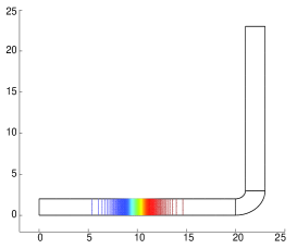
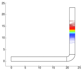
Figure 2: The wave is transmited for $R=2$, $w=2$ and $v_{0}=0.25$, while $v_{c}\approx 0.29$.

The initial kinetic energy of the kink, which is located in the straight section, far away from the curved region and from the domain edge to avoid interference from the boundaries, with initial velocity $v_{0}$, is

$$T_{0}=\int_{0}^{\ell}\int_{-w/2}^{w/2}\frac{1}{2}\phi_{t}^{2}~{}du~{}ds=4wv_{0}^{2}.$$ (9)

When $T_{0}$ is large enough to overcome the potential $U$ the wave crosses the barrier running along the channel as shown in the contour-plot sequence of Fig. 2. The minimal velocity for the kink to cross the barrier is calculated by comparing the kinetic energy $T_{0}$ to the potential energy $U$. It is approximately

$$v_{c}\approx\frac{w}{\sqrt{12}R}\sqrt{\mathrm{tanh}\frac{s_{2}-s_{1}}{2}}$$ (10)

On the other hand when the wave is not initially fast enough, the potential barrier reflects the wave and it returns with a negative velocity (see Fig. 3).

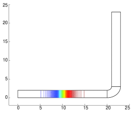
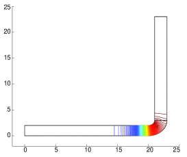
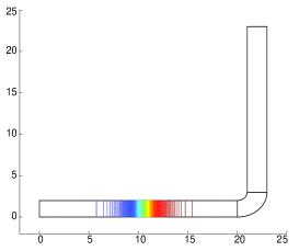
Figure 3: The wave is reflected for $R=2$, $w=2$ and $v_{0}=0.25$, while $v_{c}\approx 0.29$.

We now proceed to compare quantitatively the predictions of this simple theory with the solution of the 2D problem. We do this by plotting the phase space $(S,dS/dt)$ both for the collective variable dynamics (energy levels) and the kink position $S$ and velocity $dS/dt$ estimated from the 2D solution. The initial position of the kink is fixed well away from the curved region $20<S<20+R\pi/2$. Then the initial velocity of the soliton determines completely its trajectory as can be seen in the phase space $(S,dS/dt)$ shown in Fig. 4. When the initial velocity is lower than $v_{0}\approx 0.2$ the orbits do not cross the curved region. On the other hand for higher initial velocities the orbits span the complete circuit through the $S$ axis. Due to the existence of effective potential barrier the velocity of kink decreases in the curved segment. Fig. 4 shows that the orbits calculated from the numerical solution of the 2D system are are in very good agreement with the ones given by the collective coordinate approach.

Figure 4: Phase space $(S,dS/dt)$ of the kink position and velocity for $R=2$ and $w=2$. Comparison of simulations (continuous lines) and the collective coordinates (dashed lines).

The simple analytical approach developed above provides a good description of the kink dynamics for small velocities, otherwise the ansatz used in Eq. (6) may be too crude for large ones. In that case the kink ansatz should also depend on the variable $u$ as the contour plot of Fig. 5 shows. The distance in $s$ covered by the wave increases as $u$ decreases from $w/2$ to $-w/2$. Thus the soliton velocity depends on the level at $u$ axis and Lorenz contraction induces the different kink widths observed for different values of $u$.

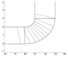
Figure 5: Contour plot of the wave at the curved section for $R=2$, $w=2$ and $v_{0}=0.20$.

The numerical simulations are done in the cartesian coordinates using the Femlab finite element software [17] to define the domain $\Omega$ and discretizing it by a triangular mesh. The time evolution has been performed with a differential equation solver.

We consider a nonlinear wave propagation in a curved planar wave guide using as a model kink solutions for the sine-Gordon equation. Specifically the domain considered $\Omega$ in the plane is made of two rectangular regions joined by a bent section of constant curvature. The transverse homogeneous Neuman boundary conditions allow us to consider a homogeneous kink solution. Following this we develop a simple collective variable theory based on the kink position. This shows that curved regions act as potential barriers for the waves in contrary to the case of Dirichlet boundary conditions. We calculate the treshold velocity for the kink to cross and it is in excellent agreement with the solutions of the full problem calculated with Femlab finite element program. The phase-space of the system matches also well the one obtained from the numerical solution.

This study shows that it is possible to trap fluxons in a Josephson junction, in the region between two successive bends. Choosing a conveniently small damping term, one may decrease the kinetic energy of the soliton as it comes into this region so that it will stay there. This feature could be applied to electronic devices for storing binary data.

C.G. and Yu. B. G. acknowledge the hospitality of the Technical University of Denmark and of the University of the Basque Country helping with all kind of facilities during the investigation period. Financial support was provided by the LOCNET Program (HPRN-CT-1999-00163), a project from the University of the Basque Country (UPV00100.310-E-14806/2002).

References

- [1] C. M. Soukoulis. Photonic Crystals and Light Localization in the 21st Century. NATO Science Series C563, Kluwer Academic, Dordrecht, Boston & London, 2001.
- [2] M.A. Reed and W.P. Kirks, editors. Nanostructure Physics and Fabrication. Academic Press, New York, 1989.
- [3] T. Shinjo, T. Okuno, R. Hassdorf, K. Shigeto, and T. Ono. Science, 289:930, 2000.
- [4] M. Kl ui, C. A. F. Vaz, J. Rothman, J. A. C. Bland, W. Wernsdorfer, G. Faini, and E. Cambril. Phys. Rev. Lett., 90:097202, 2003.
- [5] R. L. Schult, D. G. Ravenhall, and H. W. Wyld. Phys. Rev. B, 39:5476, 1989.
- [6] J. Goldstone and R. L. Jaffe. Phys. Rev. B, 45:14100, 1992.
- [7] Yu. B. Gaididei and O. O. Vakhnenko. J. Phys.: Condens. Matter, 6:32229, 1994.
- [8] A. Mekis, S. Fan, and J. D. Joannopoulos. Phys. Rev. B, 58:4809, 1998.
- [9] P. L. Christiansen and O. H. Olsen. Propagation of fluxons on a josephson line with impurities. Wave Motion, 4:163–172, 1985.
- [10] P. L. Christiansen and O. H. Olsen. Ring-shaped quasi-solitons to the two and three-dimensional sine-Gordon equation. Phys. Scripta, 20:531–538, 1979.
- [11] P. L. Christiansen and P. S. Lomdahl. Numerical study of 2 + 1 dimensional sine-Gordon solitons. Physica D, 60:482–494, 1981.
- [12] T. Harayama, P. Davis, and K. S. Ikeda. Phys. Rev. Lett., 82:3803, 1999.
- [13] A. Wallraff, A. V. Ustinov, V. V. Kurin, I. A. Shereshevsky, and N. K. Vdovicheva. Phys. Rev. Lett., 84:151, 2000.
- [14] S. F. Mingaleev, Yu. S. Kivshar, and R. A. Sammut. Phys. Rev. E, 62:5777, 2000.
- [15] Yu. B. Gaididei, S. F. Mingaleev, and P. L. Christiansen. Phys. Rev. E, 62:R53, 2000.
- [16] A. E. Leanhardt, A. P. Chikkatur, D. Kielpinski, Y. Shin, T. L. Gustavson, W. Ketterle, and D. E. Pritchrad. Phys. Rev. Lett., 89:040401, 2002.
- [17] Comsol AB. Femlab, multiphysics in matlab, June 2002. Scientific software for PDE using finite elements method.