Recurrence of fidelity in near integrable systems

Abstract

Within the framework of simple perturbation theory, recurrence time of quantum fidelity is related to the period of the classical motion. This indicates the possibility of recurrence in near integrable systems. We have studied such possibility in detail with the kicked rotor as an example. In accordance with the correspondence principle, recurrence is observed when the underlying classical dynamics is well approximated by the harmonic oscillator. Quantum revivals of fidelity is noted in the interior of resonances, while classical-quantum correspondence of fidelity is seen to be very short for states initially in the rotational KAM region.

I introduction

Qualitative dynamical behaviour of a classical system is characterized by the sensitivity of its orbits with respect to initial conditions. The sensitivity also changes with parameters of the system. If an orbit is not sensitive to initial conditions, the underlying dynamics is regular. On the other hand, for chaotic dynamics the orbit is highly sensitive to initial condition. Lyapunov exponents, which measure the rate of exponential divergence of two initially close orbits, is zero for the regular case and positive for the chaotic case. An analogous classification of dynamics is not possible in the quantum domain, since quantum theory does not accommodate the very concept of orbits.

If we associate two localized wave packets which are initially close-by in state space, overlap of these states remain invariant under unitary quantum evolution. The corresponding classical Liouville evolution of phase space densities is also a linear unitary one, but the ability to develop structures on infinitesimal scales, without the restrictions of the uncertainty principle, coexists with underlying orbit chaos. In the quantum mechanical case exponential instability of for instance the wave packet center is seen for quantized chaotic systems over a short time scale, corresponding to the Ehrenfest time scale.

One approach to quantify quantum sensitivity was initiated a while back by Peres [1] who proposed the overlap of states that are evolved from the same initial state $|\alpha\rangle$ under two Hamiltonians differing by a small perturbation. The overlap intensity, also known as fidelity, is defined as

$$f(t)=|\langle\alpha|e^{iH_{1}t/\hbar}e^{-iH_{0}t/\hbar}|\alpha\rangle|^{2}$$ (1)

where $H_{0}$ represents the Hamiltonian of an unperturbed system, $H_{1}=H_{0}+\epsilon V$ represents the perturbed system and $\epsilon$ is the perturbation parameter. Fidelity has evoked enormous interest in recent years with different interpretations. It is a measure of quantum irreversibility in the context of decoherence when the system under investigation interacts with a classically chaotic environment [2]. It is realized as polarization echo in nuclear magnetic resonance, measuring the irreversibility in many body quantum dynamics [3]. It also characterizes the loss of phase coherence in quantum computation [4].

Initial investigations by Peres [1] show that $f(t)$ is appreciable (on a time average) and its fluctuations are more for the regular case than for the chaotic case. Some of the recent studies have focused on the decay rate of $f(t)$ for chaotic systems [5]. More investigations on this topic show that while the fidelity decays on time scale $\sim 1/\epsilon^{2}$ for chaotic systems, it decays on shorter time scale $\sim 1/\epsilon$ for integrable systems [6]. In [7] the decay for integrable system is shown to have power-law behaviour.

In this paper, using perturbative approximations, we relate recurrence time of the quantum fidelity to the classical period. This indicates that recurrence of quantum fidelity would be possible in nearly integrable systems. With the kicked rotor as a dynamical model, we examine this recurrence phenomena in detail. Our numerical experiments also reveal that the evolution of fidelity exhibits a wide range of behaviour, depends on the choice of initial state.

II formulation

Let us consider an unperturbed system $H_{0}\equiv H(\omega)$, with $\omega$ being the system parameter, satisfying the eigenvalue equation

$$H_{0}|u_{n}\rangle=E_{n}|u_{n}\rangle\,.$$ (2)

Let $H_{1}\equiv H(\omega^{\prime})$ be the perturbed system where $\omega^{\prime}=\omega+\epsilon$ and $\epsilon$ is the perturbation parameter. Under a small perturbation, for the simplest zeroth order approximation to the fidelity it is sufficient to assume that the energy eigenvalues differ up to the first order of $\epsilon$ and the corresponding eigenstates remain unaffected. It is easy to see that the eigenstate changes contribute to the fidelity at an order $\epsilon$.

That is the approximation we can make for the calculation of fidelity amounts to the approximation:

$$H_{1}|u_{n}\rangle\approx\tilde{E}_{n}|u_{n}\rangle\;\;;\;\;\tilde{E}_{n}\approx E_{n}+\epsilon\;{dE_{n}\over d\omega}\,.$$ (3)

Here $dE_{n}/d\omega$ measures the rate at which $n$th level changes with the parameter. It is also known in the literature as level velocity wherein the parameter is thought of as pseudo-time. In this approximation the fidelity can be written as

$$f(t)\approx\left|\sum_{n}|c_{n}|^{2}\exp\left[-{i\epsilon t\over\hbar}\left({dE_{n}\over d\omega}\right)\right]\right|^{2}$$ (4)

where $c_{n}=\langle u_{n}|\alpha\rangle$. Note that $f(0)=1$ and we are interested in the time evolution of the fidelity. Assuming that the weighting probabilities $|c_{n}|^{2}$ are strongly centered around a mean $\bar{n}$, one can expand $dE_{n}/d\omega$ using Taylor series in $n$ around $\bar{n}$ up to the first-order correction as

$${dE_{n}\over d\omega}={dE_{\bar{n}}\over d\omega}+(n-{\bar{n}}){d^{2}E_{\bar{n}}\over dn\,d\omega}\;.$$ (5)

This gives the recurrence time

$$t_{r}=\left({2\pi\hbar\over\epsilon}\right)\left|{d^{2}E_{\bar{n}}\over dn\,d\omega}\right|^{-1}$$ (6)

such that the fidelity becomes unity when $t$ is an integer multiples of $t_{r}$. Recollecting that the classical action $S$ is quantized as $(2\pi\hbar)n=S$,

$$t_{r}={1\over\epsilon}\left|{d^{2}E_{\bar{n}}\over dS\,d\omega}\right|^{-1}\,.$$ (7)

In terms of $T=dS/dE$, the period of the classical orbit underlying the coherent state $|\alpha\rangle$, the recurrence time is thus given by a combination of simple perturbative and semiclassical approximations as

$$t_{r}={T^{2}\over\epsilon}\left|{dT\over d\omega}\right|^{-1}.$$ (8)

Thus the recurrence time of quantum fidelity is directly related to period of the underlying classical motion as well as to its variability to the relevant parameters.

III harmonic oscillator

According to the above relation, the quantum fidelity for the harmonic oscillator

$$H(\omega)={p^{2}\over 2}+{1\over 2}{\omega}^{2}q^{2}$$ (9)

with a classical period $T=2\pi/\omega$ recurs at

$$t_{r}={2\pi\over\epsilon}\,.$$ (10)

This recurrence time can also be obtained from the underlying classical dynamics by evolving an initial phase space density $\rho\,(q,p)$ which satisfies the normalization condition

$$\int\rho\,(q,p)\,dq\,dp=1\,.$$ (11)

Analogous to the quantum fidelity, we define normalized classical fidelity as

$$F(t)=\left\{\int\rho^{2}\,(q,p)\,dq\,dp\right\}^{-1}\int\rho\,(q,p)\,\rho\,(q_{2t},p_{2t})\,dq\,dp\,.$$ (12)

where $\rho\,(q_{2t},p_{2t})$ is the final phase space density which is obtained from forward time evolution of the initial density for a time $t$ with the frequency being $\omega$, followed by backward time evolution for the same time $t$ with the frequency set as $\omega^{\prime}$. The classical fidelity measures the overlap of the initial density with the final density so obtained.

If the forward time evolution of the oscillator is given by $(q,p)\rightarrow(\tilde{q},\tilde{p})$ i.e.,

$$\left[\begin{array}[]{c}\tilde{q}\\ \tilde{p}\end{array}\right]=\left[\begin{array}[]{cc}\cos(\omega t)&(1/\omega)\sin(\omega t)\\ -\omega\sin(\omega t)&\cos(\omega t)\end{array}\right]\left[\begin{array}[]{c}q\\ p\end{array}\right]\,,$$ (13)

the initial density evolves forward in time $t$ as $\rho\,(q,p)\rightarrow\rho\,(q_{t},p_{t})$ where $q_{t}$ and $p_{t}$ are given by the relation:

$$\left[\begin{array}[]{c}q_{t}\\ p_{t}\end{array}\right]=\left[\begin{array}[]{cc}\cos(\omega t)&-(1/\omega)\sin(\omega t)\\ \omega\sin(\omega t)&\cos(\omega t)\end{array}\right]\left[\begin{array}[]{c}q\\ p\end{array}\right]\,.$$ (14)

Then we consider the backward evolution for the same time $t$ with the frequency now set to $\omega^{\prime}$; $\rho\,(q_{t},p_{t})\rightarrow\rho\,(q_{2t},p_{2t})$ where $q_{2t}$ and $p_{2t}$ are given by the relation:

$$\left[\begin{array}[]{c}q_{2t}\\ p_{2t}\end{array}\right]=\left[\begin{array}[]{cc}\cos(\omega^{\prime}t)&(1/\omega^{\prime})\sin(\omega^{\prime}t)\\ -\omega^{\prime}\sin(\omega^{\prime}t)&\cos(\omega^{\prime}t)\end{array}\right]\left[\begin{array}[]{c}q_{t}\\ p_{t}\end{array}\right]\,.$$ (15)

We shall now write

$$\left[\begin{array}[]{c}q_{2t}\\ p_{2t}\end{array}\right]=\left[\begin{array}[]{cc}a&b\\ c&d\end{array}\right]\left[\begin{array}[]{c}q\\ p\end{array}\right]$$ (16)

where the elements of square matrix are obtained by combining the Eqns. (14) and (15).

If $q_{2t}=q$ and $p_{2t}=p$ for some time $t=t_{R}$, then $F(t_{R})=1$ and the classical fidelity recurs fully. This condition is given by

$$\left|\begin{array}[]{cc}a-1&b\\ c&d-1\end{array}\right|=0\,.$$ (17)

Since $(ad-bc)=1$, the above condition becomes $a+d=2$. The recurrence time $t_{R}$ then satisfies the relation

$$2\cos(\omega t_{R})\cos(\omega^{\prime}t_{R})+\left[{\omega^{2}+\omega^{\prime 2}\over\omega\omega^{\prime}}\right]\sin(\omega t_{R})\sin(\omega^{\prime}t_{R})=2\,.$$ (18)

Substituting $\omega^{\prime}=\omega+\epsilon$ and approximating $\omega^{\prime 2}\approx\omega^{2}+2\epsilon\omega$ (up to the first order of $\epsilon$), this condition reduces to

$$\cos(\epsilon t_{R})=1\;\;\;\hbox{or}\;\;\;t_{R}={2\pi\over\epsilon}\,.$$ (19)

Thus recurrence time $t_{R}$ of the classical fidelity, at this level of approximations, is identical to that of the quantum fidelity given by the Eqn.(10). This shows that recurrence of quantum fidelity for the harmonic oscillator is a manifestation of the underlying classical dynamics. If we replace $\omega$ by $i\omega$ and $\omega^{\prime}$ by $i\omega^{\prime}$, the dynamics corresponds to the unstable motion of an inverted harmonic oscillator. In this case the recurrence condition is

$$2\cosh(\omega t_{R})\cosh(\omega^{\prime}t_{R})-\left[{\omega^{2}+\omega^{\prime 2}\over\omega\omega^{\prime}}\right]\sinh(\omega t_{R})\sinh(\omega^{\prime}t_{R})=2\,.$$ (20)

Up to the first order of $\epsilon$, this condition reduces to $\cosh(\epsilon t_{R})=1$ which has only the trivial solution $t_{R}=0$. Hence there is no recurrence in the classical fidelity of the unstable oscillator.

IV kicked rotor

For further investigations on the recurrence phenomena in near integrable systems, we consider the kicked rotor whose Hamiltonian is

$$H={p^{2}\over 2}+V(q)\sum_{j}\delta(j-t)\,.$$ (21)

Here $V(q)=k\cos(2\pi q)/4\pi^{2}$ and $k$ is the kick strength - the only parameter of the system. The corresponding kick-to-kick dynamics is given by the standard map:

$$\left.\begin{array}[]{lll}p_{t+1}&=&p_{t}+(k/2\pi)\sin(2\pi q_{t})\\[6.0pt] q_{t+1}&=&q_{t}+p_{t+1}\end{array}\right\}(\hbox{mod}\;1)\,.$$ (22)

Note that the modulo operation restricts $q$ and $p$ to between $-1/2$ and $1/2$ with the opposite edges being identified. The kick-to-kick quantum dynamics is given by the quantum map:

$$|\psi_{t+1}\rangle=U_{0}|\psi_{t}\rangle\;\;;\;\;U_{0}=\exp[-ip^{2}/2\hbar]\,\exp[-iV(q)/\hbar]$$ (23)

where $U_{0}\equiv U(k)$ is the unit-time quantum propagator.

The 2-torus phase space can be quantized upon introducing periodic boundary conditions in both the canonical variables [8]. This imposes finite number, $N$, of quantum states such that $N=1/2\pi\hbar$ ($N\rightarrow\infty$ is the classical limit); we take $N=500$ for the following calculations. Since the Hamiltonian is time periodic, according to Floquet theory [9] fundamental solutions statisfy the eigenvalue equation

$$U_{0}|\phi_{n}\rangle=e^{i\phi_{n}}|\phi_{n}\rangle$$ (24)

where $\phi_{n}$ are real (between 0 and $2\pi$). If $\phi_{n}=E_{n}/\hbar$, then $E_{n}$ are called quasienergies which are analogous to the energy eigenvalues of the time-independent Hamiltonian system [10]. Correspondingly the states $|\phi_{n}\rangle$ are called quasienergy states. It is worth noting that as a consequence of hermiticity of the Hamiltonian, the quasienergy states $|\phi_{n}\rangle$ are orthogonal and they form a complete set in the $N$ dimensional space. The quasienergy spectrum can be numerically obtained by diagonalizing the matrix representation of $U$. Choosing the discrete position eigenstates $|l\rangle$ as the basis, $U$-matrix takes the form [11]

$$\langle l|U|l^{\prime}\rangle={1\over\sqrt{N}}\exp\left[-i\pi\left\{{1\over 4}-{{(l-l^{\prime})}^{2}\over N}+2NV\left({l^{\prime}\over N}\right)\right\}\right]$$ (25)

where $l,l^{\prime}=-N/2,-N/2+1,\ldots N/2-1$.

Let us consider $U_{0}$ as an unperturbed system and $U_{1}\equiv U(k+\delta k)$ as the perturbed system. Then the quantum fidelity is given by

$$f(t)=|\langle\alpha|U_{1}^{-t}U_{0}^{t}|\alpha\rangle|^{2}.$$ (26)

In accordance with our earlier approximations the eigenstates of the perturbed system are taken to be such that

$$U_{1}|\phi_{n}\rangle\approx e^{i\tilde{\phi}_{n}}|\phi_{n}\rangle\;\;;\;\;\tilde{\phi}_{n}\approx\phi_{n}+\delta k{d\phi_{n}\over dk}$$ (27)

where $d\phi_{n}/dk=\hbar^{-1}\langle\phi_{n}|dV/dk|\phi_{n}\rangle$, quantum fidelity for the kicked rotor can be approximated as

$$f(t)\approx\left|\sum_{n}|\langle\phi_{n}|\alpha\rangle|^{2}\exp\left[-{it\delta k\over\hbar}\left(d\phi_{n}\over dk\right)\right]\right|^{2}\,.$$ (28)

This gives the recurrence time as

$$t_{r}={T^{2}\over\delta k}\left|{dT\over dk}\right|^{-1}.$$ (29)

with $T$ being the classical period of the rotor.

V numerical results

The dynamical features of the standard map depends on the kick strength. In the absence of kick ($k=0$), it is just the twist map with regular dynamics. For small kick strengths ($k<1$), the phase space is predominantly regular with primary nonlinear resonance zones along $p=0$ and there are large number of smooth Kolmogorov-Arnold-Moser (KAM) tori in large $|p|$ regions on which the motion is quasiperiodic (see Fig. 1). These two distinct phase space regions are demarcated by a separatrix. In this case, the phase space is similar to that of the simple pendulum. As $k$ increases, the KAM tori are slowly destroyed and at $k\approx 1$ all the KAM tori are destroyed [12] leading to the onset of global chaos. When $k\gg 1$, the dynamics is predominantly chaotic. In this paper, we take $k=0.3$ and $\delta k=0.01$ throughout, as our interest is restricted to the near integrable regime.

To evaluate the quantum fidelity for different regions of the phase space, we take the initial state as a coherent state peaked at $(q_{0},p_{0})$, i.e., $|\alpha\rangle=|q_{0},p_{0}\rangle$. It is a minimum uncertainty (very nearly Gaussian) wave packet with equal spread $\sigma=\sqrt{\hbar/2}$ in both the canonical variables. Such an initial state on the torus can be constructed by the method devised by Saraceno [13]. The initial states we have chosen for the following computations are marked in Fig. 1.

For comparison, we also compute the classical fidelity by taking an initial phase space density to be a Gaussian

$$\rho\,(q,p)={1\over 2\pi\sigma^{2}}\exp\left[-{1\over 2\sigma^{2}}\left\{(q-q_{0})^{2}+(p-p_{0})^{2}\right\}\right]\,.$$ (30)

This density is a classical equivalent of the coherence state $|q_{0},p_{0}\rangle$ containing an ensemble of $10^{4}$ initial conditions. For the classical evolution, each point of the initial density is forward iterated using the standard map (with parameter $k$) for $t$ steps, followed by backward iteration for $t$ steps by the corresponding time reversed map, with $k$ being replaced by $k+\delta k$. This gives the final density $\rho\,(q_{2t},p_{2t})$. With this, we use a discretized version of Eqn. (12) to calculate the classical fidelity.

It should be emphasized that the recurrence of fidelity is possible only when the perturbative approximation is valid. In order to validate this approximation for different regions of the phase space, we compute phase space representation of inverse participation ratio (IPR) as

$$z(q,p)=\sum_{n}|\langle\phi_{n}|q,p\rangle|^{4}$$ (31)

such that $z^{-1}$ measures the effective number of states $|\phi_{n}\rangle$ required to construct a given region of phase space. As we see from Fig. 2, while very few states are required to construct the region near the stable fixed point, many states contribute to construct the separatrix region and rotational KAM region. In other words, low energetic part of the spectrum that corresponds to the neighborhood of stable fixed point has very low density of states; high energetic part of the spectrum that corresponds to the separatrix and KAM regions are highly dense. Generally, such simple perturbative expansions work badly for the dense spectrum. Hence the approximation is expected to be valid near the stable fixed point, and so is the recurrence of quantum fidelity. For other cases, the approximation would not be sufficient and the recurrence is not expected. As we demonstrate below, this is indeed the case. Nevertheless, for the dense spectrum, “quantum revivals” of fidelity may occur which is beyond the scope of present study, but it is under active study.

To begin with, we focus on the neighborhood of the stable fixed point. Note that Jacobian of the standard map evaluated at $(0.5,0)$ has eigenvalues $e^{\pm i\lambda}$ and $\lambda$ is obtained from the relation

$$e^{i\lambda}+e^{-i\lambda}=2\cos\lambda=2-k\,.$$ (32)

Since $\lambda$ is the frequency of the oscillatory motion in this region, the corresponding period is

$$T(k)={2\pi\over\lambda}=2\pi\left[\cos^{-1}\left({2-k\over 2}\right)\right]^{-1}$$ (33)

and we obtain the recurrence time as

$$t_{r}={2\pi\over\delta k}\sqrt{k(4-k)}\,.$$ (34)

For the parameters we have considered here ($k=0.3$,$\;\delta k=0.01$), the quantum fidelity recurs at $t_{r}=662$. If we approximate the underlying oscillatory motions by harmonic oscillators with frequencies

$$\omega=\left[\cos^{-1}\left({2-k\over 2}\right)\right]^{-1}\;\;;\;\;\omega^{\prime}=\omega+\epsilon=\left[\cos^{-1}\left({2-k-\delta k\over 2}\right)\right]^{-1}\,,$$ (35)

then $t_{r}=2\pi/\epsilon=667$.

In Fig. 3 we show the evolution of fidelity for the initial state $|0.45,0\rangle$ that is localized in the neighborhood of the stable fixed point. For initial time steps, quantum fidelity has a smooth fall-off from unity to zero. It remains nearly zero for some time and then it rises and recurs at $t=667$. This is close to the value 662 that is obtained from perturbation theory. Notice that the recurrence time matches exactly with that of the harmonic oscillator approximation. The fidelity also recurs periodically and the agreement with perturbation theory is found to be good. In addition, we find that the classical evolution exactly retraces quantum evolution. Thus, fidelity for oscillatory motion in the neighborhood of a stable fixed point exhibits very good quantum-classical correspondence.

Fig. 4 corresponds to the state which is initially placed in the interior of the primary resonance zone. In this case, the quantum fidelity almost recurs i.e, $95\%$ recurrence is observed at $t=670$. Note that this time is close to the recurrence time predicted from the harmonic oscillator approximation. Here also the perturbative approximation agrees fairly well with the actual evolution. However, unlike the previous case, classical evolution initially follows the quantum evolution and then deviates at later time steps. This shows that the observed near recurrence of fidelity is a “pure” quantum phenomena. This shows interestingly that, within the primary resonance zone, the quantum dynamics seems to be less sensitive to nonlinearity.

As we see from Fig. 5, quantum evolution is highly complex when the underlying classical motion is on the separatrix. The perturbative approximation fails and the fidelity does not recur. In this case, asymptotically the classical fidelity becomes more stable in comparison to the quantum counterpart. If we approximate unstable motion on separatrix by an inverted harmonic oscillator, classical fidelity also does not exhibit any recurrence.

Finally, we move on to the rotational KAM region of the phase space. A typical evolution of an initial state localized in this region is shown in Fig. 6. As expected, perturbative approximation fails and there are no signatures of fidelity recurrence. Although classical motion on the KAM tori is regular, we notice that quantum-classical correspondence is seen only for a short time. This may be due to enhanced quantum interference in this region of energetic rotational motion. More study on these issues is currently underway.

VI conclusion

We have shown that, within the framework of simple perturbative and semiclassical approximations, recurrence time of quantum fidelity is related to period of the classical motion. In the case of the harmonic oscillator, fidelity recurs at $t_{r}=2\pi/\epsilon$ where $\epsilon$ is the perturbation parameter. Invoking the kicked rotor as an example, we have studied in detail the recurrence phenomena for nearly integrable regimes. It is shown that quantum fidelity recurs only when the underlying classical motion is well approximated by the harmonic oscillator. This recurrence is also in accordance with the correspondence principle. Though the recurrence is not possible in other cases, quantum revival of fidelity can occur and this needs further investigation.

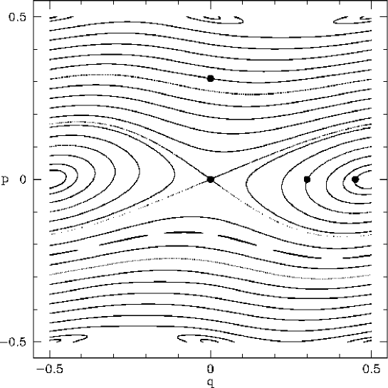
FIG. 1.: Phase space portrait of the standard map for $k=0.3$. The points $(q_{0},p_{0})=(0.45,0),(0.3,0),(0,0)$ and $(0,0.3)$, shown as solid circles, correspond to the intitial coherent states used for the quantum evolution.

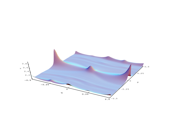
FIG. 2.: The phase space representation of the Inverse Participation Ratio $z(q,p)$ plotted for $k=0.3$.

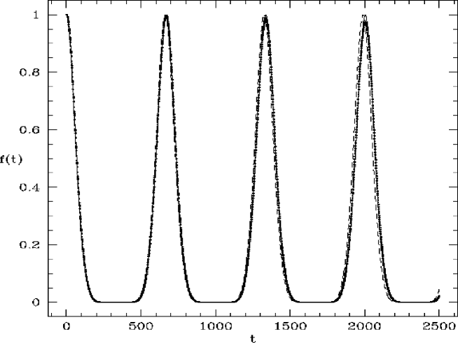
FIG. 3.: The solid line is the quantum fidelity for the initial state centered at $(0.45,0)$, near the stable fixed point, and the dashed line is the perturbative approximation (28). The corresponding classical fidelity, evaluated from Eqn. (12), is shown as dots.

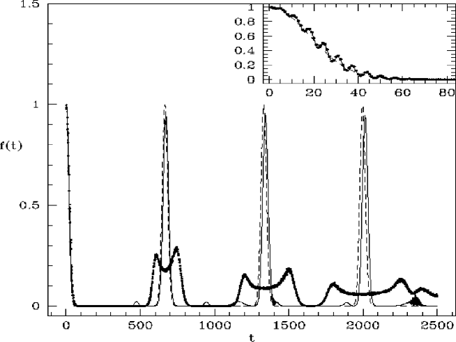
FIG. 4.: The solid line is the quantum fidelity for the initial state centered at $(0.3,0)$, in the interior of the primary resonance zone, and the dashed line is the perturbative approximation (28). For comparison, the corresponding classical fidelity is shown as dots. Inset shows the initial evolution.

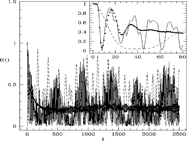
FIG. 5.: The solid line is the quantum fidelity for the initial state centered at $(0,0)$, the unstable fixed point, and dashed line is the perturbative approximation (28). Dots are the corresponding classical fidelity and the initial evolution is shown in the inset.

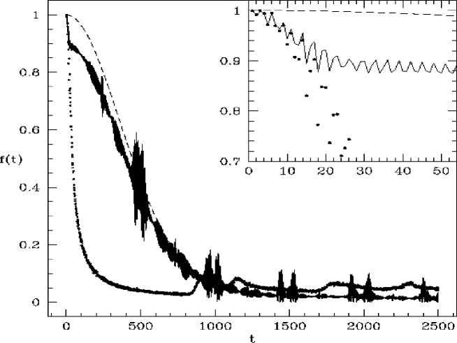
FIG. 6.: The solid line is the quantum fidelity for the initial state centered at $(0,0.3)$, on a rotational KAM curve, and the dashed line is the perturbative approximation (28). Dots are the corresponding classical fidelity and the initial evolution is shown in the inset.

REFERENCES

- [1] A. Peres, Phys. Rev. A 30, 1610 (1984).
- [2] R.A. Jalabert and H.M. Pastawski, Phys. Rev. Lett. 86, 2490 (2001); Z.P. Karkuszewski, C. Jarzynski, W.H. Zurek, quant-ph/0111002.
- [3] H.M. Pastawski, P.R. Levstein and G. Usaj, Phys. Rev. Lett. 75, 4310 (1995); G. Usaj, H.M. Pastawski and P.R. Levstein, Mol. Phys. 95, 1229 (1998).
- [4] M.A. Nielsen and I.L. Chuang, Quantum Computation and Quantum Information, Cambridge University Press, 2000.
- [5] Ph. Jacquod, P.G. Silvestrov and C.W.J. Beenakker, Phys. Rev. E 64, 055203(R) (2001); N.R. Cerruti and S. Tomsovic, Phys. Rev. Lett. 88, 054103 (2002); G. Benenti and G. Casati, quant-ph/0112060.
- [6] T. Prosen, Phys. Rev. E 65, 036208 (2002); T. Prosen and M. Znidaric, J. Phys. A 35, 1455 (2002).
- [7] Ph. Jacquod, I. Adagideli and C.W.J. Beenakker, Europhys. Letts. 61, 729 (2003).
- [8] J. Ford, G. Mantica and G.H. Ristow, Physica D 50, 493 (1991).
- [9] D.W. Jordan and P. Smith, Nonlinear Ordinary Differential Equations, Clarendon Press, Oxford 1977.
- [10] H. Sambe, Phys. Rev. A 7, 2203 (1973).
- [11] A. Lakshminarayan, Pramana J. Phys. 48, 517 (1997).
- [12] J.M. Greene, J. Math. Phys. 20, 1183 (1979).
- [13] M. Saraceno, Ann. Phys. 199, 37 (1990).