[nlin/0307004] 1 Energy trapping in the nearest neighbor model. (top) Distribution of kinetic energies as a function of time for an initial condition with all the energy 𝐸=1.28 originally in oscillator 0. (bottom) The same for 𝐸=5.12.

Energy trapping in loaded string models with

long- and short-range couplings

Ilya V. Pogorelov¹ and Henry E. Kandrup^1,2,3

¹ Department of Physics, University of Florida, Gainesville, FL 32611

² Department of Astronomy, University of Florida, Gainesville, FL 32611

³ Institute for Fundamental Theory, University of Florida, Gainesville, FL 32611

Abstract

This note illustrates the possibility in simple loaded string models of trapping most of the system energy in a single degree of freedom for very long times, demonstrating in particular that the robustness of the trapping is enhanced by increasing the ‘connectance’ of the system, i.e., the extent to which many degrees of freedom are coupled directly by the interaction Hamiltonian, and/or the strength of the couplings.

The work described here was motivated by a desire to understand the qualitative difference in dynamical behavior in systems interacting via short- and long-range couplings. In particular, how do bulk properties involving mixing and relaxation vary as the strength or the range of the interaction is increased? Considerable work has been done on systems like the Fermi-Pasta-Ulam (FPU) model, which involve only nearest neighbor couplings (see, e.g., Ford 1992). However, comparatively little is known about the phenomenology of systems which manifest longer range couplings. How does the dynamics change for high-connectance systems (see, e.g., Froeschlé 1978), which couple directly all, or almost all, the degrees of freedom?

When considering systems with longer range couplings, even the natural language in which to describe the dynamics changes. Most work on FPU-type models has involved an analysis formulated in terms of the modes of the system. However, for systems with longer range interactions it often becomes less obvious how to identify a natural set of modes. More natural, perhaps, is to consider individual degrees of freedom as fundamental, and to interpret the observed behavior in terms of those degrees of freedom.

The work described here can be viewed as a prolegomenon towards more systematic work underway which aims to study mixing properties in self-consistent systems described in the continuum limit by partial differential equations, such as the Vlasov-Poisson system of galactic astronomy, plasma physics, or charged-particle beams.

As a simple example, consider a loaded string-type model consisting of $N=16$ identical nonlinear oscillators arranged in a one-dimensional closed chain with dynamics generated by the Hamiltonian

H=\sum_{i=0}^{N-1}{\Bigl{(}}{1\over 2}p_{i}^{2}+{1\over 2}q_{i}^{2}+{1\over 4}q_{i}^{4}{\Bigr{)}}+{1\over 4}\sum_{i{\;}{\geq}{\;}j=0}^{N-1}c_{ij}{\Bigl{(}}q_{i}-q_{j}{\Bigr{)}}^{4}{\;}{\equiv}{\;}\sum_{i=0}^{N-1}H_{i}+\sum_{i{\;}{\geq}{\;}j=0}^{N-1}H_{ij},

with $q_{N}{\;}{\equiv}{\;}q_{0}$ , and view the system as a sum of $N$ individual one-degree-of-freedom Hamiltonians $H_{i}$ plus an interaction Hamiltonian $H_{int}=\sum H_{ij}$ . To explore how the dynamics depends on both the range of the interaction and the number of degrees of freedom that are coupled directly, one can then allow for three different types of couplings:

1.

a model with nearest neighbor couplings, with $c_{ij}$ nonzero only for $|i-j|=1$ , and with all nonzero $c_{ij}$ ’s assuming the same value;
2.

a maximally connected model, with all pairs coupled identically; and
3.

another long-range model, where the coupling constant decreases linearly from a fixed value $c$ for nearest neighhbors to zero strength for oscillators separated by $N/2$ ‘spaces.’

Unless otherwise specified, the computations described here assumed a coupling strength $c_{i,i+1}=1/3$ .

As a highly special, albeit interesting, initial condition, suppose that, at $t=0$ , all the system energy is deposited into a single degree of freedom, setting the kinetic energy for one of the oscillators, say oscillator $0$ , equal to the total system energy $E$ . The obvious question then is how long it takes before a sizeable fraction of the energy is transferred to the other oscillators and/or the interaction Hamiltonian.

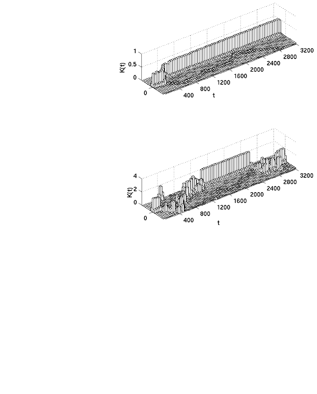
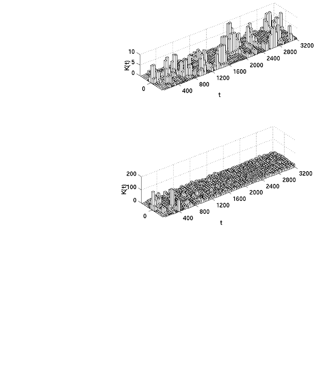
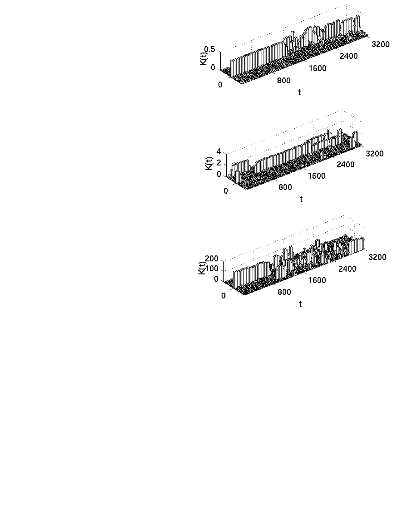
Consider first models with nearest neighbor couplings. In this case, one discovers that a significant fraction of the total energy can remain trapped in a single degree of freedom for times as long as ${\sim}{\;}10^{2}-10^{3}$ periods of uncoupled oscillations. This is, e.g., illustrated in Figs. 1 and 2, which exhibit the distribution of kinetic energies amongst the different oscillators as a function of time for four different energies. Here, as in Figs. 3 - 5, the kinetic energies have been smoothed from raw data recorded at intervals ${\delta}t=0.1$ by a box-car averaging over 400 adjacent points. The initial localization involves of course the oscillator in which the energy was originally deposited. Eventually, however, different degrees of freedom emerge as the location of this energy localization, the transitions occuring quite abruptly and with no obvious correlation between the locations of the localization prior to and following the transitions. The sojourn times also appear to be random, except that for higher energies and/or weaker coupling, the intervals between the successive transitions become shorter overall. For example, in the long-range model with linear decrease in coupling strength, reducing $c$ from $1/3$ to $1/9$ can decrease the typical duration of these intervals by as much as a factor of five. For very high energies, the localized configuration breaks down rapidly, never to appear again (see, e.g., Fig. 2, bottom panel).

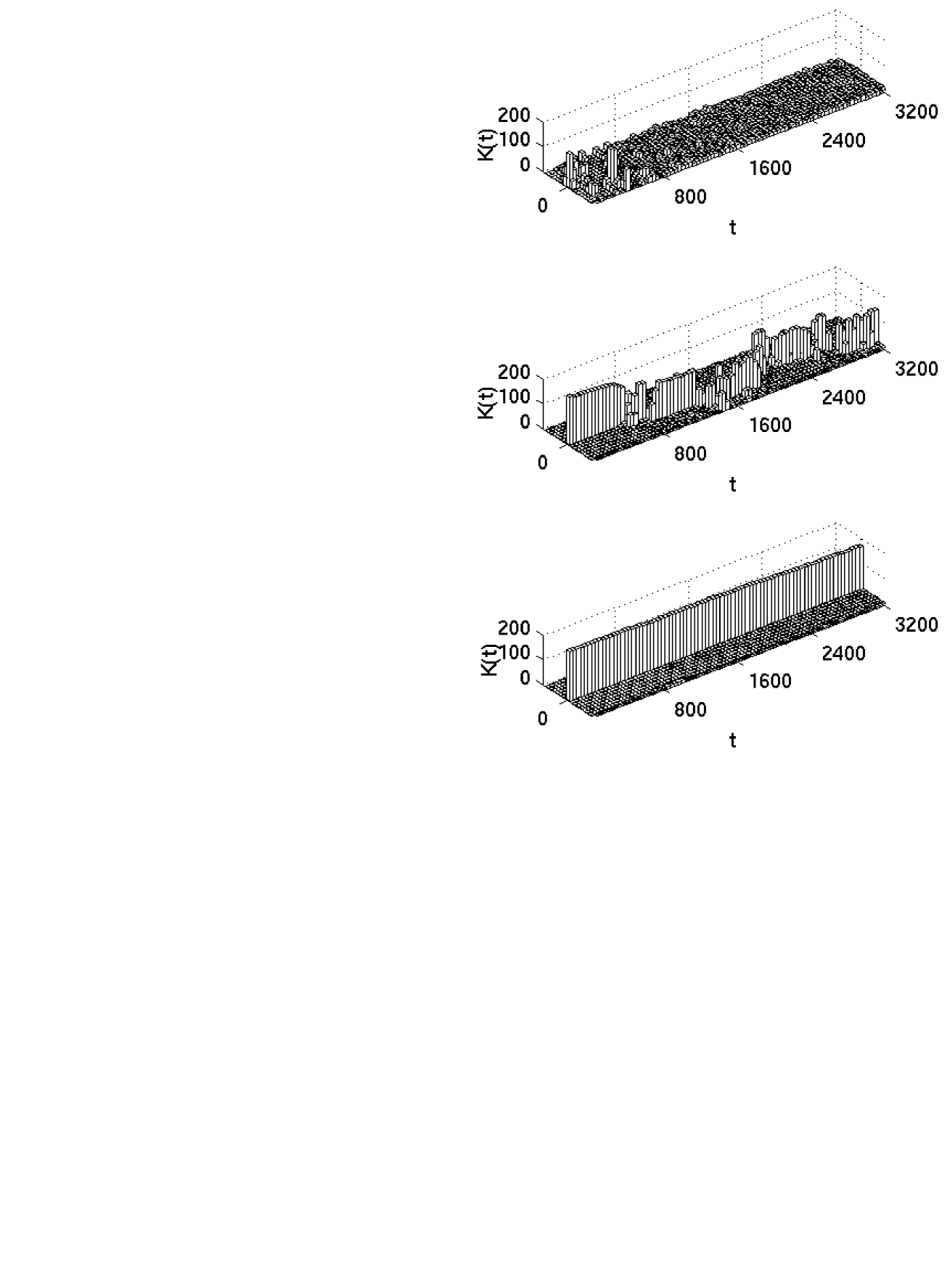
The obvious question is how this conclusion is altered for the case of longer range interactions. In particular, does increasing the range of the coupling make the energy ‘disperse’ more quickly? Here the answer is a resounding: no! Far from providing new channels for energy transfer between the degrees of freedom, long-range couplings make this energy localization, or trapping, even more robust. For every value of energy that was explored – $0.02{\;}{\leq}{\;}E{\;}{\leq}{\;}327.68$ –, localization was more robust for the models that coupled together all the degrees of freedom than for the nearest neighbor model, with the maximally connected model allowing trapping for the longest time. The degree to which a long range coupling enhances trapping can be inferred from Fig. 3, which exhibits the distribution of kinetic energies for the different oscillators for the three different models, in each case allowing for an energy $E=327.68$ . Also evident from Figs. 1 - 3 is the fact that, for all three models, the ‘trapping time’ decreases with increasing energy, a relative sharp decrease being observed for energies above $E_{*}{\;}{\sim}{\;}5-20$ , the value of which depends on the model.

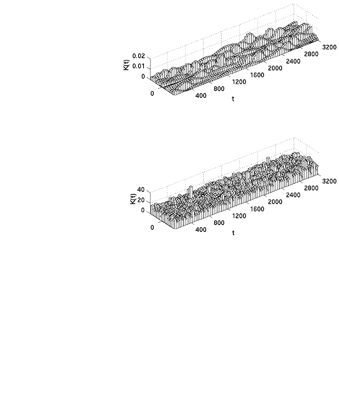
However, as illustrated by Fig. 4, localization does not emerge for ‘more generic’ initial conditions with energy distributed randomly amongst all the oscillators, so one might perhaps conjecture that this localization is a fluke reflecting a very nongeneric initial condition. It is therefore important to determine the stability of these localized configurations. In particular, one needs to determine whether, for initial conditions ‘less singular’ than $E_{0}=E$ , energy trapping persists and, if so, for how long.

These issues were addressed by considering alternative sets of initial conditions, where the initial kinetic energy of the zeroeth oscillator was assigned smaller fractions of the energy, $E_{0}=0.85E$ and $E_{0}=0.7E$ , and the remaining energy was apportioned at random in the other degrees of freedom. Putting energy into the other degrees of freedom does indeed tend to make localization less robust. However, even for $E_{0}=0.7E$ one can see distinct localization patterns that persist over hundreds of natural oscillation periods. Moreover, as before, stronger and/or longer range couplings mean that the localization persists for longer times. Decreasing the fraction of the total energy placed into the ‘trap’ results in shorter trapping times. This behavior is illustrated in Fig. 5, where different coupling types and values of $E$ are chosen so as to demonstrate the competing effects of longer range coupling and higher energy. In all three cases, the initial condition is one with 70% of the total energy deposited in oscillator 0.

The middle panel of this Figure also illustrates another interesting point: It is possible for most of the energy localized initially in a single oscillator to be deposited in two other oscillators, where it remains localized for a comparatively long time. Alternatively, as illustrated in the bottom panel of Fig. 1, an initial state which would appear to have become largely delocalized can ‘relocalize’ with most of the energy concentrated in a different oscillator.

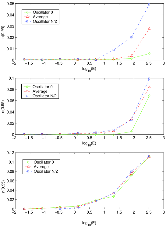
Since the efficacy of mixing is well known to differ for regular and chaotic dynamics, it is also natural to ask whether the comparatively abrupt transition from robust to less stable trapping with increasing energy $E$ correlates with a transition from (near-)regular to (more strongly) chaotic dynamics. One useful diagnostic in addressing such a transition is provided by examining the ‘complexity’ of the time series associated with some phase space variable, such as the position, momentum, or energy of one of the oscillators. One can, e.g., determine the number of frequencies required, on average, to capture some significant fraction, (say) $95\%$ , of the total power in the Fourier spectrum associated with some time series.

Such an analysis reveals that, for lower energies, the time series are very close to periodic whereas, for higher energies, any quasi-periodic approximation requires an enormous number of frequencies. There is, moreover, a strong correlation between the magnitude of the time series complexity and the rate of delocalization. The transition from very slow to considerably more rapid delocalization and the transition from very long-lived to considerably less long-lived trapping are comparably abrupt. And the complexity for the shorter range models, where localization is less robust, tends to be somewhat larger than for the time series of the longer range models. Finally, it is evident that, at least while energy remains trapped in one oscillator, the time series for the coordinate or momentum corresponding to that oscillator is typically much less complex than the the time series for the other degrees of freedom. Alternatively, at least for the case of the maximally connected model, the oscillator in the chain directly opposite from the oscillator in which the energy is localized tends to have an especially complex time series.

Examples of this behavior are exhibited in Fig. 6, which derive from orbital data recorded at intervals ${\delta}t=0.1$ for a total time $t=3200$ . In each case, $n(0.95)$ represents the fraction of frequencies required to capture 95% of the power in a time series for phase space coordinates $q_{i}$ and $p_{i}$ . The bottom curve exhibits data for the oscillator into which all the energy was originally deposited, the diamonds representing mean values obtained by computing complexities individually for $q_{0}$ and $p_{0}$ and then averaging. The top curve exhibits data for the oscillator separated by $N/2$ ‘spaces’. The middle curve was derived by computing complexities analogously for all $16$ oscillators and then constructing an average over the oscillators.

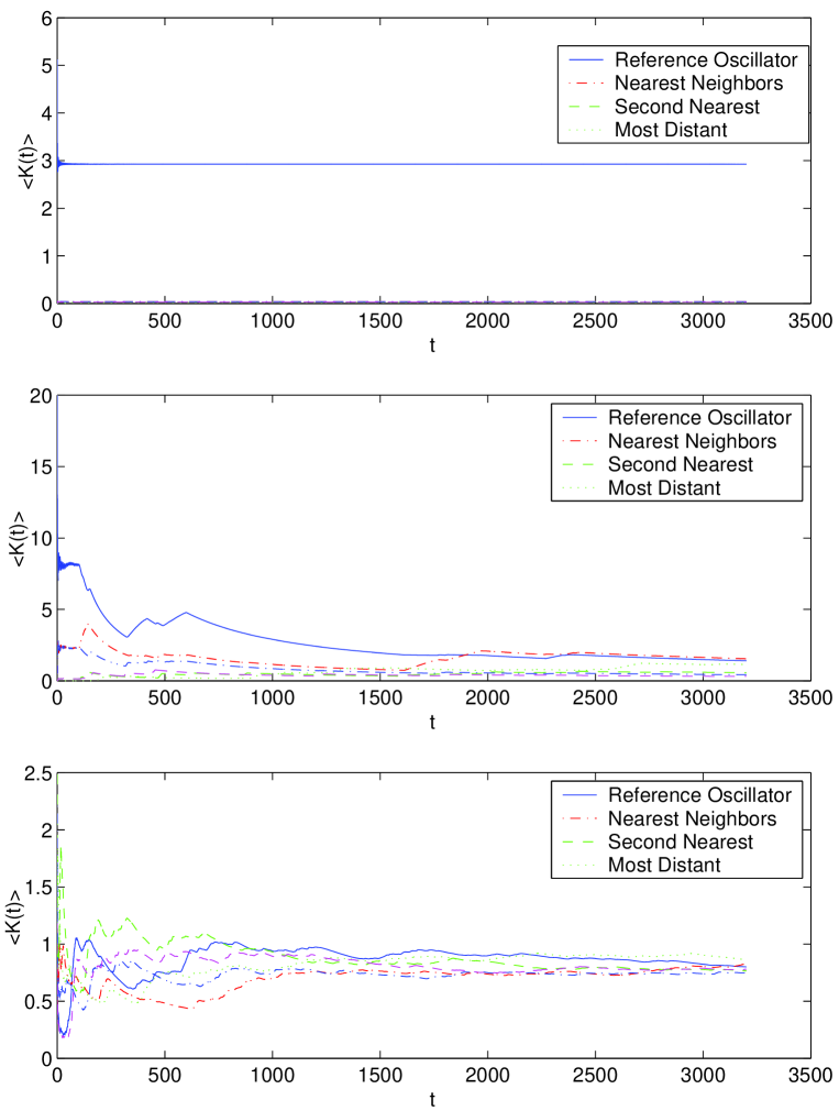
Presuming that the flow is ergodic, one would expect an eventual evolution towards a ‘well mixed’ state; and, for that reason, it is natural to determine the extent to which there is an asymptotic approach towards equipartitioning of energy at late times. For the case of random initial conditions, there are in fact clear indications of such an approach, at least in a time-averaged sense, although the time scale for this approach can be very long, $>10^{3}$ orbital periods. Obviously, though, for localized initial states there can be no such approach as long as trapping persists. However, even here there are some indications for an eventual approach towards equipartitioning for higher energies, weaker couplings, and/or shorter range interactions. Examples of an approach towards equipartitioning, or lack thereof, are provided in Fig. 7, which tracks the time-averaged kinetic energies (cf. Batt 1987)

{\langle}K(t){\rangle}={1\over n}\sum_{i=1}^{n}K(t_{i}),

with $t_{1}=0$ and $t_{n}=t$ , of several different oscillators in three representative integrations.

A number of interesting questions still remain to be addressed. For each of the different types of coupling, is there, e.g., a threshold value of energy or coupling strength signaling a transition from regularity to chaos and a comparatively rapid breakdown of localization? How does the behavior observed for $N=16$ vary as the number of degrees of freedom increases? And, perhaps most importantly, is this localization unique to one-dimensional chains? Will a similar localization persist on a two-dimensional lattice configured as a torus? Work on these questions is currently underway.

In any event, the numerical experiments performed hitherto yield three unambiguous conclusions: (1) FPU-type systems with both nearest-neighbor and longer range couplings admit states in which most of the energy remains trapped in a single degree of freedom for relatively long times. (2) The stronger the coupling in terms of range, connectance, or size of the coupling constant $c$ , the more robust is this energy trapping. (3) This trapping is more robust at lower energies, where the dynamics seems more nearly regular.

HEK was supported in part by NSF-AST-0070809.

References

Batt, J. 1987, Transport Theory Stat. Phys. 16, 763

Ford, J. 1992, Phys. Repts. 213, 271

Froeschlé, C. 1978, Phys. Rev. A 18, 277

Refer to caption — Figure 1: Energy trapping in the nearest neighbor model. (top) Distribution of kinetic energies as a function of time for an initial condition with all the energy $E=1.28$ originally in oscillator 0. (bottom) The same for $E=5.12$ .