Non–linear fractal interpolating functions of one and two variables

Abstract

We consider non–linear generalizations of fractal interpolating functions applied to functions of one and two variables. The use of such interpolating functions in resizing images is illustrated.

I Introduction

An Iterated Function System (IFS) may be used to construct fractal interpolation functions for some data barn ; ifs ; sv . The simplest example of interpolating a function $x(t)$, given data points ($t_{i},x_{i}$), $i=0,1,\ldots,N$, starts with an IFS

$$W_{n}\left(\begin{array}[]{c}t\\ x\end{array}\right)=\left(\begin{array}[]{cc}a_{n}&0\\ c_{n}&0\end{array}\right)\left(\begin{array}[]{c}t\\ x\end{array}\right)+\left(\begin{array}[]{c}e_{n}\\ f_{n}\end{array}\right).$$ (1)

The coefficients $a_{n},c_{n},e_{n}$, and $f_{n}$ determined from the conditions, for $n=1,2,\ldots,N$,

$$W_{n}\left(\begin{array}[]{c}t_{0}\\ x_{0}\end{array}\right)=\left(\begin{array}[]{c}t_{n-1}\\ x_{n-1}\end{array}\right),\qquad W_{n}\left(\begin{array}[]{c}t_{N}\\ x_{N}\end{array}\right)=\left(\begin{array}[]{c}t_{n}\\ x_{n}\end{array}\right).$$ (2)

which leads to

$$a_{n}=\frac{t_{n}-t_{n-1}}{t_{N}-t_{0}},\quad e_{n}=\frac{t_{n-1}t_{N}-t_{n}t_{0}}{t_{N}-t_{0}}\quad c_{n}=\frac{x_{n}-x_{n-1}}{t_{N}-t_{0}},\quad f_{n}=\frac{x_{n-1}t_{N}-x_{n}t_{0}}{t_{N}-t_{0}},$$ (3)

With these, the transformation of Eq. (1) can be written as

$$W_{n}(t)\equiv t^{\prime} = \frac{(t-t_{0})}{(t_{N}-t_{0})}\ t_{n}+\frac{(t-t_{N})}{(t_{0}-t_{N})}\ t_{n-1}$$

$$W_{n}(x)\equiv x^{\prime} = \frac{(t^{\prime}-t_{n-1})}{(t_{n}-t_{n-1})}\ x_{n}+\frac{(t^{\prime}-t_{n})}{(t_{n-1}-t_{n})}\ x_{n-1}$$ (4)

in which form it is apparent $W_{n}(x)\equiv x^{\prime}$ is determined by a linear (in $t$) interpolating function between the points ($t_{n-1},x_{n-1}$) and ($t_{n},x_{n}$). Graphs of fractal interpolating functions can then be made by applying the random iteration algorithm:

• initialize ($t,x$) to a point in the interval of interest

• for a set number of iterations

  • randomly select a transformation $W_{n}(t,x)$

  • plot ($t^{\prime},x^{\prime}$) $=W_{n}(t,x)$

  • set ($t,x$) $=$ ($t^{\prime},x^{\prime}$)

• end for

In this paper we consider two non–linear generalizations of such fractal interpolating functions. The first concerns how to extend the linear interpolation of Eq. (4) to higher–degree interpolations. The second generalization arises when one considers the construction of fractal interpolating functions for functions of two (or more) variables – in this case, even a linear interpolation of the form of Eq. (4), when applied to each variable, will result in a non–linear interpolating function. This has an obvious application in representing two–dimensional images, where a function of two variables (the pixel coordinates) could represent a black–and–white image (using a Boolean function), a gray–scale image (using a scalar function), or a colour image (using a vector–valued function of the three rgb [red, green, blue] values). This problem has been examined extensively in the context of image compression jaq ; comp1 ; comp2 ; mass ; in the last section we consider a related problem of using these iterated function systems to rescale images, or portions thereof.

II Functions of two variables

We first consider a function $z(x,y)$ of two variables, and examine the problem of constructing a fractal interpolating function from the data $x_{i},y_{j},z_{i,j}$, where $i=0,1,\ldots,M$, $j=0,1,\ldots,N$, and $z_{i,j}\equiv z(x_{i},y_{j})$. To this end, consider the transformation

$$W_{mn}(x) = a_{mn}x+e_{mn}$$

$$W_{mn}(y) = c_{mn}y+f_{mn}$$

$$W_{mn}(z) = A_{mn}x+B_{mn}y+C_{mn}xy+D_{mn}$$ (5)

We then impose, for $m=1,2,\ldots,M$ and $n=1,2,\ldots,N$ the conditions

$$W_{mn}\left(\begin{array}[]{c}x_{M}\\ y_{N}\end{array}\right)=\left(\begin{array}[]{c}x_{m}\\ y_{n}\end{array}\right),\qquad W_{mn}\left(\begin{array}[]{c}x_{0}\\ y_{0}\end{array}\right)=\left(\begin{array}[]{c}x_{m-1}\\ y_{n-1}\end{array}\right),$$ (15)

$$W_{mn}(z_{M,N})=z_{m,n},\qquad W_{mn}(z_{M,0})=z_{m,n-1},\qquad W_{mn}(z_{0,N})=z_{m-1,n},\qquad W_{mn}(z_{0,0})=z_{m-1,n-1}.$$ (16)

The coefficients turn out to be

$$a_{mn} = \frac{x_{m}-x_{m-1}}{x_{M}-x_{0}},\qquad e_{mn}=\frac{x_{0}x_{m}-x_{m-1}x_{M}}{x_{0}-x_{M}},$$

$$c_{mn} = \frac{y_{n}-y_{n-1}}{y_{N}-y_{0}},\qquad f_{mn}=\frac{y_{0}y_{n}-y_{n-1}y_{N}}{y_{0}-y_{N}},$$

$$A_{mn} = \frac{(z_{m,n-1}-z_{m-1,n-1})y_{N}-(z_{m,n}-z_{m-1,n})y_{0}}{(x_{M}-x_{0})(y_{N}-y_{0})},$$

$$B_{mn} = \frac{(z_{m-1,n}-z_{m-1,n-1})x_{M}-(z_{m,n}-z_{m,n-1})x_{0}}{(x_{M}-x_{0})(y_{N}-y_{0})},$$

$$C_{mn} = \frac{z_{m,n}-z_{m,n-1}-z_{m-1,n}+z_{m-1,n-1}}{(x_{M}-x_{0})(y_{N}-y_{0})},$$

$$D_{mn} = \frac{z_{m,n}x_{0}y_{0}-z_{m,n-1}x_{0}y_{N}-z_{m-1,n}x_{N}y_{0}+z_{m-1,n-1}x_{N}y_{N}}{(x_{M}-x_{0})(y_{N}-y_{0})}.$$ (17)

With these, the transformation of Eq. (LABEL:twovar) can be written as

$$W_{mn}(x)\equiv x^{\prime} = \frac{(x-x_{0})}{(x_{M}-x_{0})}\ x_{m}+\frac{(x-x_{M})}{(x_{0}-x_{M})}\ x_{m-1}$$

$$W_{mn}(y)\equiv y^{\prime} = \frac{(y-y_{0})}{(y_{N}-y_{0})}\ y_{n}+\frac{(y-y_{N})}{(y_{0}-y_{N})}\ y_{n-1}$$

$$W_{mn}(z)\equiv z^{\prime} = \frac{(x^{\prime}-x_{m-1})(y^{\prime}-y_{n-1})}{(x_{m}-x_{m-1})(y_{n}-y_{n-1})}\ z_{m,n}+\frac{(x^{\prime}-x_{m})(y^{\prime}-y_{n-1})}{(x_{m-1}-x_{m})(y_{n}-y_{n-1})}\ z_{m-1,n}+$$

$$+ \frac{(x^{\prime}-x_{m-1})(y^{\prime}-y_{n})}{(x_{m}-x_{m-1})(y_{n-1}-y_{n})}\ z_{m,n-1}+\frac{(x^{\prime}-x_{m})(y^{\prime}-y_{n})}{(x_{m-1}-x_{m})(y_{n-1}-y_{n})}\ z_{m-1,n-1}$$ (18)

in which form it is apparent $W_{mn}(z)\equiv z^{\prime}$ is determined by a function implementing a linear interpolation over the grid ($x_{m-1},y_{n-1}$), ($x_{m-1},y_{n}$), ($x_{m},y_{n-1}$), and ($x_{m},y_{n}$).

III Quadratic interpolating functions

The interpolating functions considered up to now have used a linear interpolating formula between adjacent points to construct the IFS. In this section we indicate how this can be generalized to quadratic interpolations.

III.1 Functions of one variable

For a function $x(t)$ of one variable, using data points ($t_{i},x_{i}$), $i=0,1,\ldots,N$, consider the transformations

$$W_{n}(t) = a_{n}t+e_{n}$$

$$W_{n}(x) = c_{n}t+d_{n}t^{2}+f_{n}$$ (19)

and impose the conditions, for $n=2,3,\ldots,N$,

$$W_{n}\left(\begin{array}[]{c}t_{0}\\ x_{0}\end{array}\right)=\left(\begin{array}[]{c}t_{n-2}\\ x_{n-2}\end{array}\right),\qquad W_{n}\left(\begin{array}[]{c}t_{M}\\ x_{M}\end{array}\right)=\left(\begin{array}[]{c}t_{n-1}\\ x_{n-1}\end{array}\right),\qquad W_{n}\left(\begin{array}[]{c}t_{N}\\ x_{N}\end{array}\right)=\left(\begin{array}[]{c}t_{n}\\ x_{n}\end{array}\right).$$ (20)

The point $t_{M}$ is determined as

$$t_{M}=\frac{(t_{n-1}-t_{n-2})}{(t_{n}-t_{n-2})}\ t_{N}+\frac{(t_{n-1}-t_{n})}{(t_{n-2}-t_{n})}\ t_{0}$$ (21)

with corresponding point $x_{m}$. The coefficients of the IFS are determined as

$$a_{n} = \frac{t_{n}-t_{n-2}}{t_{N}-t_{0}}$$

$$e_{n} = \frac{t_{N}t_{n-2}-t_{0}t_{n}}{t_{N}-t_{0}}$$

$$c_{n} = \frac{x_{n}(t_{0}^{2}-t_{m}^{2})+x_{n-1}(t_{N}^{2}-t_{0}^{2})+x_{n-2}(t_{m}^{2}-t_{N}^{2})}{(t_{N}-t_{0})(t_{N}-t_{m})(t_{m}-t_{0})}$$

$$d_{n} = \frac{x_{n}(t_{m}-t_{0})+x_{n-1}(t_{0}-t_{N})+x_{n-2}(t_{N}-t_{m})}{(t_{N}-t_{0})(t_{N}-t_{m})(t_{m}-t_{0})}$$

$$f_{n} = \frac{x_{n}t_{m}t_{0}(t_{m}-t_{0})+x_{n-1}t_{N}t_{0}(t_{0}-t_{N})+x_{n-2}t_{N}t_{m}(t_{N}-t_{m})}{(t_{N}-t_{0})(t_{N}-t_{m})(t_{m}-t_{0})}$$ (22)

with which the transformation can be written as

$$W_{n}(t)\equiv t^{\prime} = \frac{(t-t_{0})}{(t_{N}-t_{0})}\ t_{n}+\frac{(t-t_{N})}{(t_{0}-t_{N})}\ t_{n-2}$$

$$W_{n}(x)\equiv x^{\prime} = \frac{(t^{\prime}-t_{n-1})(t^{\prime}-t_{n-2})}{(t_{n}-t_{n-1})(t_{n}-t_{n-2})}\ x_{n}+\frac{(t^{\prime}-t_{n})(t^{\prime}-t_{n-2})}{(t_{n-1}-t_{n})(t_{n-1}-t_{n-2})}\ x_{n-1}$$ (23)

$$+ \frac{(t^{\prime}-t_{n-1})(t^{\prime}-t_{n})}{(t_{n-2}-t_{n-1})(t_{n-2}-t_{n})}\ x_{n-2}$$

In this form we see that a quadratic (in $t^{\prime}$) interpolating function is used between the points ($t_{n},x_{n}$), ($t_{n-1},x_{n-1}$), and ($t_{n-2},x_{n-2}$).

III.2 Functions of two variables

We next consider a function $z(x,y)$ of two variables, and construct a fractal interpolating function which employs a quadratic interpolation between points. To this end, consider the transformation

$$W_{mn}(x) = a_{mn}x+e_{mn}$$

$$W_{mn}(y) = c_{mn}y+f_{mn}$$

$$W_{mn}(z) = A_{mn}x^{2}y^{2}+B_{mn}x^{2}y+C_{mn}x^{2}+D_{mn}xy^{2}+E_{mn}xy+F_{mn}x+G_{mn}y^{2}+H_{mn}y+I_{mn}$$ (24)

We then impose, for $m=2,3,\ldots,M$ and $n=2,3,\ldots,N$, the conditions

$$W_{mn}\left(\begin{array}[]{c}x_{M}\\ y_{N}\end{array}\right)=\left(\begin{array}[]{c}x_{m}\\ y_{n}\end{array}\right),\qquad W_{mn}\left(\begin{array}[]{c}x_{M}\\ y_{M}\end{array}\right)=\left(\begin{array}[]{c}x_{m-1}\\ y_{n-1}\end{array}\right),\qquad W_{mn}\left(\begin{array}[]{c}x_{0}\\ y_{0}\end{array}\right)=\left(\begin{array}[]{c}x_{m-2}\\ y_{n-2}\end{array}\right),$$ (37)

$$W_{mn}(z_{N,N})=z_{m,n},\qquad W_{mn}(z_{N,m})=z_{m,n-1},\qquad W_{mn}(z_{N,0})=z_{m,n-2},$$

$$W_{mn}(z_{m,N})=z_{m-1,n},\qquad W_{mn}(z_{m,m})=z_{m-1,n-1}\qquad W_{mn}(z_{m,0})=z_{m-1,n-2}$$

$$W_{mn}(z_{0,N})=z_{m-2,n},\qquad W_{mn}(z_{0,m})=z_{m-2,n-1}\qquad W_{mn}(z_{0,0})=z_{m-2,n-2}$$ (38)

The points $x_{M}$ and $y_{M}$ are determined as

$$x_{M} = \frac{(x_{m-1}-x_{m-2})}{(x_{m}-x_{m-2})}\ x_{M}+\frac{(x_{m-1}-x_{m})}{(x_{m-2}-x_{m})}\ x_{0}$$

$$y_{M} = \frac{(y_{n-1}-y_{n-2})}{(y_{n}-y_{n-2})}\ y_{N}+\frac{(y_{n-1}-y_{n})}{(y_{n-2}-y_{n})}\ y_{0},$$ (39)

along with the corresponding $z$ points. The coefficients of the IFS can then be determined, by which the transformation of Eq. (38) can be written as

$$W_{mn}(x)\equiv x^{\prime} = \frac{(x-x_{0})}{(x_{M}-x_{0})}\ x_{m}+\frac{(x-x_{M})}{(x_{0}-x_{M})}\ x_{m-1}$$

$$W_{mn}(y)\equiv y^{\prime} = \frac{(y-y_{0})}{(y_{N}-y_{0})}\ y_{n}+\frac{(y-y_{N})}{(y_{0}-y_{N})}\ y_{n-1}$$

$$W_{mn}(z)\equiv z^{\prime} = \frac{(x^{\prime}-x_{m-2})(x^{\prime}-x_{m-1})(y^{\prime}-y_{n-2})(y^{\prime}-y_{n-1})}{(x_{m}-x_{m-2})(x_{m}-x_{m-1})(y_{n}-y_{n-2})(y_{n}-y_{n-1})}z_{m,n}+$$ (40)

$$+ \frac{(x^{\prime}-x_{m-2})(x^{\prime}-x_{m-1})(y^{\prime}-y_{n-2})(y^{\prime}-y_{n})}{(x_{m}-x_{m-2})(x_{m}-x_{m-1})(y_{n-1}-y_{n-2})(y_{n-1}-y_{n})}z_{m,n-1}+$$

$$+ \frac{(x^{\prime}-x_{m-2})(x^{\prime}-x_{m-1})(y^{\prime}-y_{n})(y^{\prime}-y_{n-1})}{(x_{m}-x_{m-2})(x_{m}-x_{m-1})(y_{n-2}-y_{n})(y_{n-2}-y_{n-1})}z_{m,n-2}+$$

$$+ \frac{(x^{\prime}-x_{m})(x^{\prime}-x_{m-2})(y^{\prime}-y_{n-1})(y^{\prime}-y_{n-2})}{(x_{m-1}-x_{m})(x_{m-1}-x_{m-2})(y_{n}-y_{n-1})(y_{n}-y_{n-2})}z_{m-1,n}+$$

$$+ \frac{(x^{\prime}-x_{m})(x^{\prime}-x_{m-2})(y^{\prime}-y_{n-2})(y^{\prime}-y_{n})}{(x_{m-1}-x_{m})(x_{m-1}-x_{m-2})(y_{n-1}-y_{n-2})(y_{n-1}-y_{n})}z_{m-1,n-1}+$$

$$+ \frac{(x^{\prime}-x_{m})(x^{\prime}-x_{m-2})(y^{\prime}-y_{n})(y^{\prime}-y_{n-1})}{(x_{m-1}-x_{m})(x_{m-1}-x_{m-2})(y_{n-2}-y_{n})(y_{n-2}-y_{n-1})}z_{m-1,n-2}+$$

$$+ \frac{(x^{\prime}-x_{m})(x^{\prime}-x_{m-1})(y^{\prime}-y_{n-2})(y^{\prime}-y_{n-1})}{(x_{m-2}-x_{m})(x_{m-2}-x_{m-1})(y_{n}-y_{n-2})(y_{n}-y_{n-1})}z_{m-2,n}+$$

$$+ \frac{(x^{\prime}-x_{m})(x^{\prime}-x_{m-1})(y^{\prime}-y_{n})(y^{\prime}-y_{n-2})}{(x_{m-2}-x_{m})(x_{m-2}-x_{m-1})(y_{n-1}-y_{n})(y_{n-1}-y_{n-2})}z_{m-2,n-1}+$$

$$+ \frac{(x^{\prime}-x_{m})(x^{\prime}-x_{m-1})(y^{\prime}-y_{n})(y^{\prime}-y_{n-1})}{(x_{m-2}-x_{m})(x_{m-2}-x_{m-1})(y_{n-2}-y_{n})(y_{n-2}-y_{n-1})}z_{m-2,n-2}$$

Although tedious to work out, the generalization of the preceding considerations to higher–order interpolating functions is straightforward in principle.

IV Image Scaling

As an application of the preceding, in this section we consider the task of rescaling a colour image. This is a natural problem for an interpolating function of two variables ($x,y$) interpreted as pixel coordinates – the function ${\bf\vec{z}}(x,y)$ in this case will be a vector–valued function having three components representing the rgb value of the pixel specifying the amount of red, green, and blue present.

The procedure used to scale an image of size $M$ pixels wide by $N$ pixels high is as follows. We first read in the rgb values of each pixel of the image, and use that as the data to construct a fractal interpolating function ${\bf\vec{z}}(i,j)$, where $i=1,2,\ldots,M$ and $j=1,2,\ldots,N$. To then resize the image, so that the resulting image is of size $s_{x}M\times s_{y}N$, we construct a new fractal interpolating function ${\bf\vec{z}}\,^{\prime}(i,j)={\bf\vec{z}}(s_{x}i,s_{y}j)$. Applying the random iteration algorithm to ${\bf\vec{z}}\,^{\prime}(i,j)$, choosing independently a transformation index ($i,j$) at each stage, will then result in the rescaled image. The generalization of this procedure to rescale a portion of an image is straightforward.

As examples of the results of this procedure, consider the figures in the Appendix. We start with the image appearing in Fig. 1, and zoom in on the area of the face. The result appears in Fig. 2, together with a comparison done using a simple linear interpolation scheme. Zooming further into the area of the eye results in Fig. 3, again with a comparison of the result of a simple linear interpolation. Generally, the number of iterations needed in the random iteration algorithm to produce acceptable images is of the order of $s_{x}M\times s_{y}N$, where the original image is of size $M\times N$. Also, while slower, the quadratic fractal interpolating function typically produces, for the same number of iterations, a “smoother” looking image than the corresponding linear interpolating function. However, as with all interpolation schemes, there comes a point where such higher–order interpolating formulas actually start to produce worse results due to an artificially high sensitivity to fluctuations in the data.

Some informal tests of this procedure seems to indicate that better results are obtained for images of people, natural scenery, etc., as opposed to those containing lettering, simple geometric shapes, and similar constructs. This might be expected, given the general fractal nature of such objects in nature. However, as with all interpolating functions, it is important to remember that no structural information beyond that of the original image is being provided (for example, one could not zoom in on the face of Fig. 1 to such a degree as to see individual skin pores).

The preceding demonstrates that these non–linear fractal interpolating functions of two variables can be used in principle to represent images. It would be interesting to extend these considerations to the case of partitioned iterated function systems, upon which much work has been done with respect to compressing images jaq . Work along these directions is in progress.

Scaling of figures

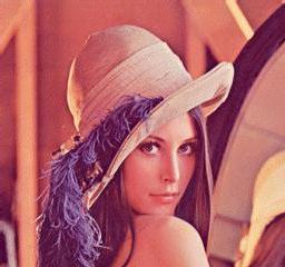
Figure 1: Original figure

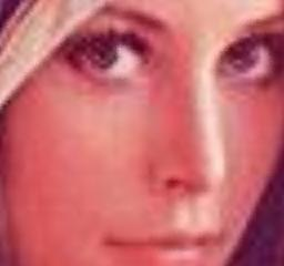
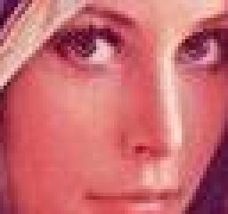
Figure 2: Enlargement of the area around the face of Fig. 1 via a) a fractal interpolation function b) a linear interpolation

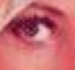
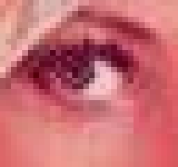
Figure 3: Enlargement of the area around the eye of Fig. 1 via a) a fractal interpolation function b) a linear interpolation

References

• (1) M. F. Barnsley, Fractals Everywhere (Academic Press, San Diego, CA, 1993)
• (2) H. O. Peitgen, H. Jürgens, and D. Saupe, Chaos and Fractals – New Frontiers of Science (Springer Verlag, New York, 1992).
• (3) H. O. Peitgen and D. Saupe, The Science of Fractal Images (Springer Verlag, New York, 1988).
• (4) A. Jacquin, IEEE trans. on Image Processing, January, 1992.
• (5) M. Barnsley, L. Hurd, and L. Anson, Fractal Image Compression (A. K. Peters, New York, 1993).
• (6) Y. Fisher (editor), Fractal Image Compression: Theory and Application (Springer Verlag, New York, 1995).
• (7) P. R. Massopust, Fractal Functions, Fractal Surfaces and Wavelets (Academic Press, San Diego, CA, 1994).