Effects of a nonlinear perturbation on dynamical tunneling in cold atoms.

Abstract

We perform a numerical analysis of the effects of a nonlinear perturbation on the quantum dynamics of two models describing non-interacting cold atoms in a standing wave of light with a periodical modulated amplitude $A(t)$. One model is the driven pendulum, considered in ref.[1], and the other is a variant of the well-known Kicked Rotator Model. In absence of the nonlinear perturbation, the system is invariant under some discrete symmetries and quantum dynamical tunnelling between symmetric classical islands is found. The presence of nonlinearity destroys tunnelling, breaking the symmetries of the system. Finally, further consequences of nonlinearity in the kicked rotator case are considered.

Tunneling is one of the most typical features of quantum mechanics, concerning oscillations between states that cannot be connected in the classical Hamiltonian dynamics by real trajectories. The original formulation of the problem involved states separated by potential barriers: the relevant features are semiclassically explained in terms of complex solutions of Hamilton equations for one-dimensional systems [2], while a proper treatment in higher dimensions is considerably subtler even when integrability is preserved [3]. Recently a novel kind of tunneling, involving transitions between classically separated regions in the presence of a non trivial structure of the phase space, has attracted considerable attention, both theoretically [4, 5, 6, 7], and experimentally [8, 1, 9]. In particular a large fraction of these papers focus on physical settings realized with cold atoms in optical potentials. The recent widespread interest and experimental activity in Bose-Einstein condensation [10] suggest to check whether the presence of Gross-Pitaevskii nonlinearities [11] deeply influences the characteristic features of dynamical tunneling. Such a question was already raised and analyzed in the framework of the kicked oscillator [12], where it was observed how the nonlinear terms typically destroys quantum effects induced by symmetry [13, 14]. The paper is organized as follows: we firstly give a few details and fix notations for the class of models we are going to consider, then analyze two cases: a driven pendulum and the kicked rotator; in the last section we briefly reconsider pioneering work made on the nonlinear kicked rotator [15, 16] and supplement it with novel results for the quantum resonant case.

I General setting.

We will consider models described by the following hamiltonian

$$H=H_{O}+V(\vartheta,t)=\frac{p^{2}}{2}+A(t)cos\vartheta,$$ (1)

where $p$ and $\vartheta$ are canonical momentum and position coordinates respectively, expressed in scaled dimensionless units, and $A(t)$ is a periodic function of time. Under appropriate choices of the function $A(t)$, the quantum version of this model describes an ensemble of non-interacting cold atoms in presence of a standing wave with a periodically modulated amplitude $A(t)$. The connection between the scaled variables $\vartheta,p$ and the physical ones $\vartheta^{\prime},p^{\prime}$ is $\vartheta=2k_{L}\vartheta^{{}^{\prime}}$ and $p={{\mathchoice{\hbox{\raise 5.06941pt\hbox to0.0pt{\kern 1.3802pt\vrule width=2.76042pt,height=0.1pt,depth=0.1pt\hss}\hbox{$\displaystyle k$}}}{\hbox{\raise 5.06941pt\hbox to0.0pt{\kern 1.3802pt\vrule width=2.76042pt,height=0.1pt,depth=0.1pt\hss}\hbox{$\textstyle k$}}}{\hbox{\raise 3.54857pt\hbox to0.0pt{\kern 0.96614pt\vrule width=1.93228pt,height=0.1pt,depth=0.1pt\hss}\hbox{$\scriptstyle k$}}}{\hbox{\raise 2.5347pt\hbox to0.0pt{\kern 0.6901pt\vrule width=1.3802pt,height=0.1pt,depth=0.1pt\hss}\hbox{$\scriptscriptstyle k$}}}}}p^{{}^{\prime}}/2k_{L}\hbar$ ( where $k_{L}$ is half of the wave vector of the standing wave and  $\textstyle k$ is the effective Planck constant $[\vartheta,p]=-i{\mathchoice{\hbox{\raise 5.06941pt\hbox to0.0pt{\kern 1.3802pt\vrule width=2.76042pt,height=0.1pt,depth=0.1pt\hss}\hbox{$\displaystyle k$}}}{\hbox{\raise 5.06941pt\hbox to0.0pt{\kern 1.3802pt\vrule width=2.76042pt,height=0.1pt,depth=0.1pt\hss}\hbox{$\textstyle k$}}}{\hbox{\raise 3.54857pt\hbox to0.0pt{\kern 0.96614pt\vrule width=1.93228pt,height=0.1pt,depth=0.1pt\hss}\hbox{$\scriptstyle k$}}}{\hbox{\raise 2.5347pt\hbox to0.0pt{\kern 0.6901pt\vrule width=1.3802pt,height=0.1pt,depth=0.1pt\hss}\hbox{$\scriptscriptstyle k$}}}}$)[17].

FIG. 1.: Poincaré section of an ensemble of classical particles for the driven pendulum. The initial ensemble is uniformly distributed in $|p|<10$, $\theta\in[-\pi,\pi[$; the values of $p$ and $\theta$ are taken at intervals multiples of the period $\tau$.

We consider two possible choices for the periodic function $A(t)$:

• The first model is the driven pendulum. The amplitude $A(t)$ is that reported in [1], i.e. $-2\alpha\cos^{2}(\pi t)$; the period $\tau$ of time modulation is 1 and the parameter $\alpha$ depends on some physical quantities of the system, kept fixed in experiments, such as the ac Stark shift amplitude, the electric field strength and the dipole momentum of the atom.

• The second model is a variant of the well-known Kicked Rotator model [18, 17], where the amplitude $A(t)$ is a sum of $\delta$ functions of period $\tau$, $k\cos\vartheta\sum_{n=0}^{n=+\infty}\delta(t-n\tau)$. The parameter $k$ measures the kick strength.

FIG. 2.: (a) The momentum distributions at times $t=0$ and (b) $t=56\tau$ for one rotor with zero quasi-momentum. The values of the parameters are $\alpha=10.0$, $N=128$, $L=500$. (c) The correspondent tunnelling oscillations of the first moment. Time is measured in number of periods.

Owing to the time dependence of the amplitude $A(t)$, in the Kicked Rotator time can be treated as a discrete variable, measured in intervals of the period $\tau$, and the evolution is discrete; in the driven pendulum instead, time is a continuous variable.

The two models present some analogies. In both models the potential $V(\vartheta,t)$ is periodic both in time and space with period $\tau$ and $2\pi$ respectively. Moreover, the two models share some symmetries: time-reversal ($(\vartheta,p,t)\to(\vartheta,-p,-t)$) and parity ($(\vartheta,p,t)\to(-\vartheta,-p,-t)$).

The quantum Hamiltonian operator of the unperturbed system is obtained from the Hamiltonian (1) replacing the classical canonical variables with the correspondent operators $\hat{\vartheta}$ and $\hat{p}=-i\hbar\partial/\partial\hat{\vartheta}$.

Space and time periodicity are conveniently dealt with by using Bloch Floquet Theory. As the potential commutes with spatial translation of $2\pi$, the quantized momentum gets eigenvalues on a discrete lattice $p=\hbar n+\beta$, $n\in{\bf Z}$ and where $\beta$, called the quasimomentum, is the analogous of the Bloch phase in solid state physics [19]. In the present paper we choose $\hbar=1$ (see the former discussion about choice of units), so that the quasimomentum takes values in the interval $[0,1)$ (the analogous of the first Brillouin zone).

Quasi-momentum is preserved during quantum evolution and parameterizes a single quantum rotor, fixing the origin of the discrete lattice in momentum space. The evolution of an ensemble of non interacting atoms can be modelled by a superposition of the evolutions of independent rotors.

Because of the invariance of the quantum evolution operator under time translation by an interval $\tau$ ($U(t+\tau)=U(t)$), an evolution operator $U_{\tau}$ over one period can be defined, called Floquet operator. The eigenvalues of Floquet operator are $e^{-i\frac{\epsilon\tau}{\hbar}}$, where the real quantities $\epsilon$, independent from $\tau$, are called quasi-energies. The quasi-energy spectrum is invariant under translation over $2\pi\hbar/\tau$. Quasi-energy plays the same role of energy in systems with continuous time variable.

Concerning the discrete symmetries we mentioned, note that changing the sign of $p$ means to change the sign of the integer part of $p$ ($[p]=n\to-n$) and to replace the fractional part $\{p\}$ of $p$ by $1-\{p\}$ ($\beta\to 1-\beta$). Therefore only rotors with $\beta=0$ or $\beta=\frac{1}{2}$ are invariant with respect to these discrete symmetries; rotors with $\beta\neq 0,\frac{1}{2}$ mix each others: a rotor labelled by $\beta$ is mapped to another rotor labelled by $\beta^{\prime}=1-\beta$.

Now we discuss some feature of quantum dynamical tunneling for the two cases we selected, also considering the effect of Gross-Pitaevskii nonlinearities.

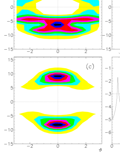
FIG. 3.: (a),(b),(c) Three Floquet eigenstates involved in the dynamics of the system; (d) the Fourier spectrum of $\langle p(t)\rangle$. The dashed horizontal line determines the limit of the dominant frequencies: the five higher peaks emerge.

II The driven pendulum.

Firstly we analyze the unperturbed system (1) without the nonlinear term, which is the theoretical setting for experimental data reported in ref.[1].

Note that, in the experimental results reported in [1], the momentum is measured in units of $2k_{L}\hbar$, which correspond to the scaled momentum $p$ divided by ${\mathchoice{\hbox{\raise 5.06941pt\hbox to0.0pt{\kern 1.3802pt\vrule width=2.76042pt,height=0.1pt,depth=0.1pt\hss}\hbox{$\displaystyle k$}}}{\hbox{\raise 5.06941pt\hbox to0.0pt{\kern 1.3802pt\vrule width=2.76042pt,height=0.1pt,depth=0.1pt\hss}\hbox{$\textstyle k$}}}{\hbox{\raise 3.54857pt\hbox to0.0pt{\kern 0.96614pt\vrule width=1.93228pt,height=0.1pt,depth=0.1pt\hss}\hbox{$\scriptstyle k$}}}{\hbox{\raise 2.5347pt\hbox to0.0pt{\kern 0.6901pt\vrule width=1.3802pt,height=0.1pt,depth=0.1pt\hss}\hbox{$\scriptscriptstyle k$}}}}\approx 2.08$.

The classical trajectories are obtained by a numerical integration of the Hamilton equations with fourth-fifth order Runge-Kutta method.

In Fig.1 the Poincaré surface of section for positions $\vartheta$ and momenta $p$ of an ensemble of classical particles is shown for the value $\alpha=10.5$: the time evolution of 1000 initial conditions, uniformly distributed in the square $|p|<10$, $\vartheta\in[-\pi,\pi[$, is recorded at 100 subsequent modulation periods. The symmetries of the system under the transformations $\vartheta\to-\vartheta$ and $p\to-p$ are clear. A pair of stable fixed points of period two $(\vartheta_{0}=0;p_{0}=\pm 8.65)$ are present. The stability islands, formed by regular trajectories surrounding the fixed points, are time-reversed images of each other.

FIG. 4.: The momentum distributions at times $t=0$ and (b) $t=10\tau$ in a system of 101 $\beta$-rotors, with $\beta$ equally spaced in the interval $0.4\leq\beta\leq 0.6$. The values of the parameters are $\alpha=10.5$, $N=128$, $L=500$. (c) The correspondent tunnelling oscillations. Time is measured in number of periods.

Since the Hamiltonian operator is non autonomous, the exact Floquet operator of a quantum rotor, with fixed quasi-momentum $\beta$, is given by a Dyson expansion. In the numerical simulation we use the lowest order split method [20]. The Floquet operator is approximated by an ordered product of evolution operators on a small intervals of time $\Delta t=\tau/L$, with $L$ integer:

$$\begin{array}[]{l}{\hat{U}}_{\tau}(\beta)=T\exp^{-i\int_{0}^{\tau}\left(\hat{H}_{0}+\hat{V}(\hat{\vartheta};t)\right)}\\ \approx\prod_{k=1}^{L}\exp^{-i\hat{H}_{0}\frac{\Delta t}{2}}\exp^{-i\hat{V}(\hat{\vartheta};t)\Delta t}\exp^{-i\hat{H}_{0}\frac{\Delta t}{2}}\\ =\prod_{k=1}^{L}\exp^{-i\frac{\tau}{4L}(\hat{n}+\beta)^{2}}\exp^{-i\frac{\tau}{L}2\alpha\cos^{2}\left(\pi\frac{\tau}{L}k\right)\cos\hat{\vartheta}}\\ \ \ \ \ \ \exp^{-i\frac{\tau}{4L}(\hat{n}+\beta)^{2}}.\\ \end{array}$$ (2)

We use a finite base of dimension $N$: the discrete momentum eigenvalues belong to the finite lattice $p=(m-\frac{N}{2})+\beta$ and the continuous angle variable is approximated by $\vartheta=\frac{2\pi}{N}(m-1)$ with $m\in{\bf Z},1\leq m\leq N$.

We start by considering the case of a simple rotor, with quasimomentum $\beta=0$.

In fig. 2 the evolution of the first moment and the correspondent momentum distribution are shown for $\alpha=10$. The initial state is a coherent state centered in one of the classical symmetric islands:

$$f(p)=C\exp^{-ip\vartheta_{0}}\exp^{-\delta^{2}(p-p_{0})^{2}},$$ (3)

where the constant $\delta$ is $\sqrt{1/2}$ and $C$ a normalization factor. In the simulations we use $\hbar=1$, $\vartheta_{0}=0$ and $p_{0}=8.525$.

FIG. 5.: (a)$\langle p(t)\rangle$ for $u=5,\alpha=10,N=128$; (b) $\langle p(t)\rangle_{u}-\langle p(t)\rangle_{0}$ versus t, for $u=3$(solid line),$7$(dashed line),$10$(dotted line).Time is measured in number of periods.

It can be seen that the maximum of the distribution probability oscillates periodically between the two symmetric values $+p_{0}$ and $-p_{0}$. In fig.2(b) the probability density is shown at time $t=56\tau$ corresponding to a negative value of $\langle p\rangle$: its maximum is peaked at $n=-9$. As we already remarked, for $\beta=0$ the quantum system is invariant with respect to parity $\hat{P}$ and time inversion $\hat{T}$ and dynamical tunnelling between the symmetric classical stable regions is present, marked by quasi-periodical oscillations of the first moment between symmetric positive and negative values (approximately $\langle p\rangle\approx\pm 6$). For values of quasimomenta $\beta$ different from $0$ or $1/2$, exact quantum symmetries are broken and periodical oscillations are damped and then suppressed. The damping of oscillations is faster for values of $\beta$ far from 0 and 1/2.

The time evolution of the first moment can be expanded in terms of Floquet eigenstates as:

$$\langle p(t)\rangle=\sum_{j,l}c_{j}(0)c^{*}_{l}(0)\exp^{-\frac{i}{\hbar}t(\phi_{j}-\phi_{l})}\sum_{n}n\chi_{j}(n)\chi^{*}_{l}(n)$$ (4)

where the Floquet eigenfunctions $\chi_{j}(n)$ are expressed in momentum representation, the phases $\phi_{j,l}$ are the correspondent eigenvalues (connected to quasi-energies by $\phi=\tau\epsilon$) and the squared modulus of the coefficients $c_{j}(0)=\langle\chi_{j}|\psi(0)\rangle$ gives the overlap of the eigenfunction $|\chi_{j}\rangle$ with the initial state. As it can be seen from (4), the Fourier frequencies $\omega_{j,l}$, in which the periodic motion can be decomposed, are separations between two Floquet eigenvalues ($\omega_{j,l}=\phi_{j}-\phi_{i}$). The dominant frequencies $\omega_{j,l}$ correspond to Floquet eigenstates that more contribute to the dynamics, having an high overlap with the initial state.

FIG. 6.: The separation time $T$ between $P_{u}$ and $P_{0}$, when $|P_{u}(T)-P_{u=0}(T)|$ exceeds the value $\Delta$ versus $u$. Starting from above, the six curves correspond to $\Delta=0.2,0.1,0.05,0.02,0.01,0.005$. In the inset a log-log plot is shown.

The Floquet eigenfunctions and eigenphases are evaluated by a numerical diagonalization of the operator.

By using a finite basis (the momentum is discretized using $N$ points), the Floquet operator is reduced to a finite matrix $N\times N$ and it is calculated as follow. The columns of the Floquet operator in the momentum representation are obtained by evolving over one period $\tau$ the momentum eigenstates. Owing to the finiteness of the basis, the evolution of the momentum eigenstates initially localized on the edges of the basis is affected by errors. To overcome this problem, we calculate the Floquet operator using a basis of double dimension $\tilde{N}=2N$, so that the variable $p$ takes discrete values in the interval $p\in[-N+1,N]$. Then we extract from the matrix $\tilde{N}\times\tilde{N}$ a nonunitary submatrix of dimension $N$ in which $p$ varies in the range $[-\frac{N}{2}+1+,\frac{N}{2}]$. The disadvantage of using a nonunitary matrix is to find some eigenvalues inside the unitary circle. Nevertheless, the number of nonunitary eigenphases and the errors can be reduced by increasing the dimensions of the bases $N$ and $\tilde{N}$.

The pairs of eigenfunctions $(\chi_{j},\chi_{i})$ that dominate the dynamics of the system are selected by three conditions [21]: a) the maximum presence probability $\bar{p}$ inside the region where the classical stable islands lie (i.e. $|n|<10$); b) the maximum overlapping probability of each eigenfunction with the initial state, $P_{j}=|\langle\chi_{j}|\psi(0)\rangle|^{2}$; c) the maximum mutual overlapping probability between the two eigenfunctions, $P_{j}P_{i}$. In fig.3(a),(b),(c) three Floquet eigenstates verifying the conditions $\bar{p}_{j}>0.5,P_{j}>0.07$ and $P_{j}P_{i}>0.0049$ are shown.

Fourier analysis of $\langle p(t)\rangle$, with a resolution of $2\pi/512\approx 0.0123$, reveals five dominant frequencies ($\omega_{1}=0.0859;\omega_{2}=0.1841;\omega_{3}=0.3559;\omega_{4}=0.4909;\omega_{5}=1.1167$). A part of the spectrum around zero is represented in fig.3 (d). The dominant frequencies are the peaks higher than the dashed horizontal line.

The differences between the eigenphases of the eigenfunctions shown in fig.3 ($\phi_{a}=4.4579,\phi_{b}=4.1035,\phi_{c}=3.9198$) correspond to the frequencies of the spectrum, marked by arrows: $\omega_{2}=\phi_{b}-\phi_{c}$, $\omega_{3}=\phi_{a}-\phi_{b}$, $\omega_{4}=\phi_{a}-\phi_{c}$.

Up to now we have considered quantum evolution corresponding to a fixed quasimomentum (that furthermore respects quantum symmetries): we now consider the evolution of a distribution of rotors with different quasimomenta $\beta$, each evolving with the operator (2) with a fixed quasi-momentum $\beta$[22]: $\psi(p,0)=f(p)\delta_{{n},{[p]}}$. The initial momentum distribution $f(p)$ is a coherent state peaked in the center of one of the two classical islands of fig.1, as in (3).

During the evolution each $\beta$-rotor evolves independently and the mean value of the observables of the system is an average over different rotors. The time evolution of the momentum distribution and of the mean value of $\hat{p}$ has been calculated. The data for $\alpha=10.5$ are shown in fig.4. The spreading in quasi-momentum is $\Delta\beta=0.2$ around the value $\beta=\frac{1}{2}$, which preserves the symmetries. The oscillations of $\langle p(t)\rangle$ correspond to the tunnelling of the quantum state between the two symmetric islands in the classical phase space. Note that, as in the experimental data [1], during time evolution, the momentum distribution of the system maintains its maximum localized in the starting island, in the region of positive momenta (see the momentum distribution in fig.4(b), corresponding to a minimum value of the average momentum).Therefore, in consequence of the average over different rotors, the oscillations of $\langle p(t)\rangle$ do not reach negative values, for which higher values of probability density in regions of negative momenta are needed.

Moreover the spreading in quasi-momentum can reproduce the decay of the oscillations in time. In accordance with [7], we have also verified that the decay of oscillations is faster if the dispersion in $\beta$ is increased.

As it can be seen from short-period oscillations in fig.4(c), the behaviour of $\langle p(t)\rangle$ is a superposition of tunnelling oscillations with slightly different frequencies, because the spreading in quasimomenta corresponds to a spreading of the dominant frequencies of the motion.

We now study the influence of a Gross-Pitaevskii nonlinearity in the dynamics: where Schrödinger operator is modified by adding a nonlinear term dependent on the squared modulus of the wave function of the system, $u|\psi|^{2}$. The approximate expression of the evolution operator becomes:

$$\begin{array}[]{l}{\hat{U}}_{\tau}(\beta)\approx\prod_{k=1}^{L}\hat{R}\left(\frac{\tau}{L}\right)\exp^{-i\frac{\tau}{L}2\alpha\cos^{2}\left(\pi\frac{\tau}{L}k\right)\cos\vartheta}\hat{R}\left(\frac{\tau}{L}\right)\\ \hat{R}\left(\frac{\tau}{L}\right)=\exp^{-i\frac{\tau}{4L}(\hat{n}+\beta)^{2}}\exp^{-i\frac{\tau}{2L}u|\psi_{n}|^{2}}\\ \end{array}$$ (5)

The multiplicative factor $\exp^{-i\frac{\tau}{2L}u|\psi_{n}|^{2}}$ breaks the symmetries of the system.

In presence of the nonlinearity term, the tunnelling oscillations of the first moment loose periodicity in time and are progressively suppressed at long times (see fig.5(a)). In fig.5(b) the difference between the first moment of the unperturbed system and that of the perturbed one is shown for three values of the nonlinear parameter $u$: $u=3$ (solid line), $u=7$ (dashed line), $u=10$ (dotted line).

FIG. 7.: Classical phase space of the Standard Map (8) for $K=2.21$ with islands of accelerator modes. The phase space is symmetric under space and time inversion.

We have also calculated the time-averaged first moment $P(t)=\frac{1}{t}\sum_{t^{\prime}=0}^{t-1}\langle p(t^{\prime})\rangle$ for fifty values of $u$ equally spaced in the interval $0<u<10$ and we have compared the value of $P_{u}$ with $P_{0}$ in absence of nonlinearity.

In fig.6 the time $T$ at which the quantity $|P_{u}(T)-P_{u=0}(T)|$ exceeds the fixed value $\Delta$ versus the nonlinear parameter $u$ is shown; each curve corresponds to a different value of the parameter $\Delta$ from 0.2 to 0.005. The intervals of time $T$ decrease algebraically with respect to $u$ with the law $T=B/u^{A}$. In table 1 the power-law exponents $A$ and the constants $B$ are shown for different parameters $\Delta$.

III Kicked Rotator Model.

The Hamiltonian of the classical system is:

$$H=\frac{p^{2}}{2}+k\cos\vartheta\sum_{n=0}^{+\infty}\delta(t-n\tau)$$ (6)

The correspondent classical map is the well-known Standard Map [23], defined on the cylinder:

$$\left\{\begin{array}[]{cc}p_{n+1}=p_{n}+k\cos\vartheta_{n}&\\ \vartheta_{n+1}=\vartheta_{n}+\tau p_{n+1}&mod(2\pi)\end{array}\right.$$ (7)

After the scaling of the variable $p$ ($p^{{}^{\prime}}=\tau p/2$) and the introduction of the parameter $K=\tau k/2$, the map can be symmetrized and reduced on the 2-torus $[0,2\pi[\times[-\pi,\pi[$:

$$\left\{\begin{array}[]{cc}\vartheta_{n+1}^{-}=\vartheta_{n}^{+}+p^{{}^{\prime}}_{n}&\\ p^{{}^{\prime}}_{n+1}=p_{n}+K\cos\vartheta_{n+1}^{-}&mod(2\pi)\\ \vartheta_{n+1}^{+}=\vartheta_{n+1}^{-}+p^{{}^{\prime}}_{n+1}&mod(2\pi)\end{array}\right.$$ (8)

where the signs $+$ and $-$ refer to instants after and before the $n$-th and $n+1$-th kicks.

The classical system depends only on the parameter $K$. For $K\geq K_{c}\approx 0.97$ the system undergoes a transition to global chaos, the last K.A.M. curve breaks and unbounded diffusion in action space takes place. Nevertheless even for $K>>1$ some small stability islands survive in the classical phase space, correspondent to accelerator modes [23, 24, 25].

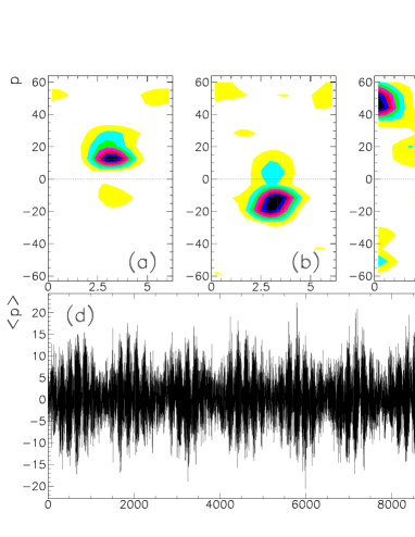
FIG. 8.: Husimi distribution of the state vector at times (a)t=800$\tau$, (b)t=900$\tau$, (c)t=8400$\tau$. (d) Tunnelling oscillations of $\langle p(t)\rangle$. Time is measured in number of periods.

In fig.7 the classical phase space of the map (8) for $K=2.21$ with the stability islands of accelerator modes is shown.

FIG. 9.: (a) A section of the eigenphases spectrum vs $k$ of the Floquet operator. Three eigenvalues for each values of $k$ are represented. (b),(c),(d) The momentum distribution of the three correspondent eigenfunctions for $k=45.02$. (e),(f),(g) The three correspondent eigenfunctions for $k=45.05$. (h),(i),(l) The three correspondent eigenfunctions for $k=45.08$.

There are two periodic orbits of period two: one formed by the pair of fixed points $(\pi,\pm 0.7656)$ and the other by the pair $(0,\pm 2.3714$). The points of each periodic orbits are symmetric respect to $p=0$. They are surrounded by stability islands inside which the dynamics of the system is regular; each island is delimited by K.A.M. curves, which cannot be crossed. During the evolution, ensembles of points initially located inside the islands centered in $(\pi,\pm 0.7656)$ do not mix with those located inside the islands centered in $(0,\pm 2.3714)$.

The invariance of the system under space reflection and time inversion can be seen clearly from the structure of the phase space.

The quantum version of the system is a variant of the Kicked Rotator Model [26], described by the Floquet operator:

$${\hat{U}}_{\tau}=\hat{R}\hat{K}\hat{R}=e^{-i\frac{\tau}{4}(\hat{n}+\beta)^{2}}e^{-ik\cos\vartheta}e^{-i\frac{\tau}{4}(\hat{n}+\beta)^{2}}.$$ (9)

(the kicked rotator corresponds to quasimomentum $\beta=0$).

For values of $\tau=4\pi M/N$ (with $M,N\in{\bf N}$) the kicked rotator undergoes a quantum resonance [27], where the spectrum acquires a band structure, yielding ballistic transport (see also [28]).

Having set $\hbar=1$, the parameters $\tau$ and $k$ are scaled by $\hbar$ with respect to the classical ones ($\tau=\tau_{cl}\hbar$ and $k=k_{cl}/\hbar$). Therefore the quantum parameter $\tau$ plays the role of $\hbar$; the classical limit of the system in obtained by the limits $\tau\to 0$, $k\to\infty$ and $K=k\tau=const.$

For $\beta=0$ or $\beta=\frac{1}{2}$ the system is invariant respect to parity $\hat{P}$ and time inversion $\hat{T}$, as in the former case. Therefore the Floquet eigenstates belong to invariant subspaces with respect to the discrete symmetries; for example they can be classified in two classes: odd or even with respect to parity [29, 30].

In the following we fix the value of $\beta=0$ and analyze first the kicked rotator for a resonant value of $\tau$ and then for a generic value of $\tau$.

A Resonant case.

Under the resonance condition $\tau=4\pi M/N$, the quantum system is periodic of period $N$, if $M$ or $N$ is even [31]. Therefore the quantum system can be reduced on a torus and its Floquet operator becomes a unitary finite matrix of dimension $N\times N$. Exact eigenfunctions can be calculated.

The discrete momentum eigenvalues are $p^{{}^{\prime}}=n=m-N/2$, with $m$ integer, varying in the interval $1\leq m\leq N$. To make a comparison between the quantum system and the classical one on the torus, the classical variable $p$ has to be rescaled by the factor $2/\tau$, i.e. $p^{{}^{\prime}}=\frac{2}{\tau}p$. Note that in the following figures the apex of the quantum variable $p^{{}^{\prime}}$ is omitted.

In fig.8 the first moment of $\hat{p}$ and the Husimi function of the momentum distributions at different times are shown for $M=1,N=128$ and $k=4.42/\tau$ ($\tau\approx 0.098$ and $k=45.022$). For the chosen value of $\tau$, the stable periodic orbits of the classical map (8) correspond to orbits $(\pi,\pm 15.6)$ and $(0,\pm 48.3)$ in the quantum phase-space. The chosen initial state is a coherent state (3) centered in ($\vartheta_{0}=0,p^{{}^{\prime}}_{0}=\frac{2}{\tau}*0.766\approx 15.605$). Periodic tunnelling oscillations between the two symmetric islands centered in $\pm p^{{}^{\prime}}_{0}$ take place.

The tunnelling oscillations are not suppressed even for long times. The calculation of $\langle p(t)\rangle$ in fig.8(d) is carried on for $10^{6}$ modulation periods.

Note that at $t=8400\tau\approx 824.668$, when $\langle p(t)\rangle$ assumes a maximum value, the quantum state is mainly localized in the island to the upper bound of the torus, centered approximately at $p^{{}^{\prime}}_{0}\approx\pm 48.3098$ (see fig.8(c)). As already said, the classical evolution of ensembles of points located in the islands centered in $p_{0}\approx\pm 2.4(p^{{}^{\prime}}_{0}\approx\pm 48.3)$ is independent from the evolution of points inside the islands centered in $p_{0}\approx\pm 0.8(p^{{}^{\prime}}_{0}\approx\pm 15.6)$, in one of which the initial wave packet is localized.

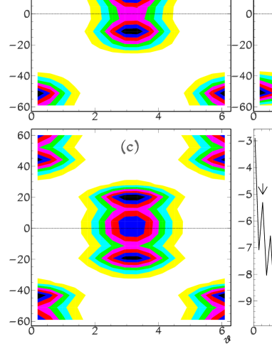
FIG. 10.: (a),(b),(c) The Husimi distribution of three eigenfunctions of the Floquet operator. (d) A section of the Fourier spectrum of $\langle p(t)\rangle$.

The quantum evolution instead couples structures that are independent in the classical system. In fact some eigenfunctions of the Floquet operator, involved in the dynamics, have high probability in both the pairs of islands (see fig.10 (a),(b),(c)).

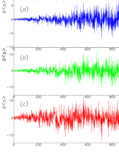
FIG. 11.: Suppression of periodical oscillations of the first moment $\langle p(t)\rangle$ in the presence of nonlinear perturbation ((a) $u=5$, (b) $u=10$, (c) $u=20$). The difference $\Delta\langle p(t)\rangle$ is plotted. The values of the parameters are $\tau=4\pi/128$, $k=4.42/\tau,N=128,L=2000$.

In fig.9(a) a portion of the spectrum of the Floquet eigenphases versus $k$ is shown. An avoided crossing can be seen, close to the value of $k$ used in the calculations of this section, i.e. $k=\frac{2K}{\tau}\approx 45.022$. The corresponding eigenfunctions were selected by having a support in the region $|n|\leq 25$ greater than $0.4$. The region $|n|\leq 25$ corresponds to the classical portion of the phase space $|p|=|\frac{\tau}{2}n|\leq 1.227$, in which the stability islands centered in $p_{0}\approx\pm 0.7656$ lie. Owing to the invariance properties of the system, the eigenfunctions localized in regular regions of the classical phase space occur in doublets of states with opposite symmetries and nearly degenerate eigenvalues; wave packets localized in the symmetric islands of stability are formed by symmetric or antisymmetric combinations of such doublets. In fig.9 (c),(d) an example of a quasi-degenerate doublet for $k=45.02$ is shown; the Husimi function of one state of this doublet is plotted in fig.10(b).

The dynamical tunnelling can be explained by a three states model [30]. In fig.9(b)-(l) the three eigenfunctions involved in the tunnelling process for three different values of $k$ are shown. Fixing a value of $k$, the three states that take part in the dynamical tunnelling are a doublet of quasi- degenerate states with opposite symmetry, localized in regular islands, and a third state localized in the chaotic region outside the stability islands ((b) for $k=45.02$,(e) for $k=45.05$,(l) for $k=45.08$). It is the chaotic state that enhance dynamic tunnelling between stability islands.

By varying $k$, the chaotic eigenstate (fig.9(b) for $k=45.02$) mixes itself with the state of the doublet sharing the same symmetry (fig.9(d) for $k=45.02$) until a complete exchange between the two states happens (fig.9(h) and fig.9(l) for $k=45.08$)[6, 30].

Beside the triplet of states shown in fig.9, there are other Floquet eigenstates that contribute to the behaviour of the first moment (4) at fixed $k$; the separations between their eigenvalues correspond to the frequencies found by the decomposition of $\langle p(t)\rangle$ in Fourier components.

The frequencies mostly contributing to the motion are revealed by peaks of the power spectrum of $\langle p(t)\rangle$, represented in fig.10(d) for the parameter $k\approx 45.022$. The spectrum has been calculated with a resolution of $\Delta\omega=2\pi/2^{18}\approx 0.000024$. The three frequencies marked by arrows are $\omega_{1}=0.000057\pm 0.000012,\ \ \omega_{2}=0.000321\pm 0.000012,\ \ \omega_{3}=0.001040\pm 0.000012$; $\omega_{1}$, $\omega_{2}$ and $\omega_{3}$ correspond to the difference between eigenphases of three doublets of quasi-degenerate eigenfunctions: $\omega_{1}=\phi_{a}-\phi_{a^{\prime}}=5.501869-5.502808$, $\omega_{2}=\phi_{b^{\prime}}-\phi_{b^{\prime}}=2.449073-2.448753$ and $\omega_{3}=\phi_{c^{\prime}}-\phi_{c^{\prime}}=4.733879-4.732833$, where $\phi_{a},\ \phi_{b},\ \phi_{c}$ are the phases of the eigenfunctions plotted in fig.10(a),10(b),10(c) respectively. These eigenfunctions have a support $\bar{p}$ in the region $|n|\leq 25$ greater than 0.45 and an overlap probability with the initial state $P_{j}$ greater than 0.01 ($P_{j}P_{i}>0.0001$).

Also in this case we may consider the effect of a nonlinear perturbation $u|\psi|^{2}$ in the Hamiltonian operator. The effect of this nonlinear perturbation on the quantum dynamics of the Kicked Rotator has already been studied in ref.[15, 16] but only in non resonant cases.

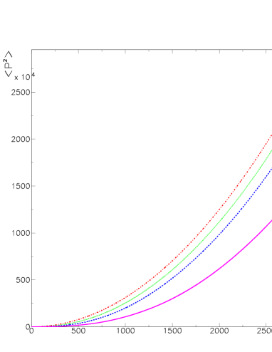
FIG. 12.: Second moment vs time, measured in numbers of periods for different values of the nonlinearity: starting from above, $u=0$ dashed-dotted line, $u=5$ dotted line, $u=10$ dashed line, $u=20$ full line. The values of the parameters are $\tau=4\pi$, $k=2.5,N=16384,L=2000$

Since the perturbation depends continuously on time through the wave function $\psi$ of the system, the time evolution operator $\hat{R}$ between the kicks is approximated as a product of evolution operators on small intervals of time $\tau/L$ ($L$ is the number of small steps):

$$\hat{R}=\prod_{i=1}^{L}e^{-i\frac{\tau}{4L}n^{2}}e^{-i\frac{i}{2}\frac{\tau}{L}|\psi_{n}|^{2}}$$ (10)

The effect of a nonlinear perturbation is to break the symmetries of the system thus destroying tunnelling. In fig.11 the difference between the first moment of the unperturbed system ($u=0$) and that of the perturbed one $\Delta\langle p(t)\rangle=\langle p(t)\rangle_{u}-\langle p(t)\rangle_{0}$ is plotted for $u=5,10,20$.

We have also analyzed the effect of the nonlinear perturbation on the second moment. In analogy with what has been found for the kicked harmonic oscillator under the resonance condition[14], in the presence of the nonlinear perturbation the growth of the second moment is slower than in the kicked rotator, even if it remains ballistic ($\langle p^{2}(t)\rangle=c(\beta)t^{2}$). In fig.12 the second moment vs time is shown: the four curves correspond to $u=0,5,10,20$ starting from above. This persistence of resonant behaviour once the nonlinear term is switched on (at least on our observation time scale) is somehow surprising, and we hope further theoretical analysis will reveal its significance (i.e. if it not suppressed on longer time scales).

B Generic case.

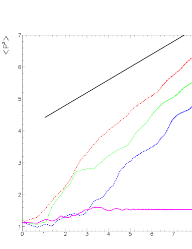
FIG. 13.: Suppression of dynamical localization of the time averaged second moment $P_{int}^{2}(t)$ in the presence of nonlinear perturbation (starting from below, $u=0$, full line, $u=5$, dashed line, $u=10$ dotted line, $u=20$, dashed-dotted line). The parameters values are $\tau=1$, $k=2.5,N=128,L=2000$.

We consider the kicked rotator for $\tau=1$ and analyze the effect of the nonlinear perturbation on the first and second moment. For this value of $\tau$ the system is far from the classical limit and displays quantum localization.

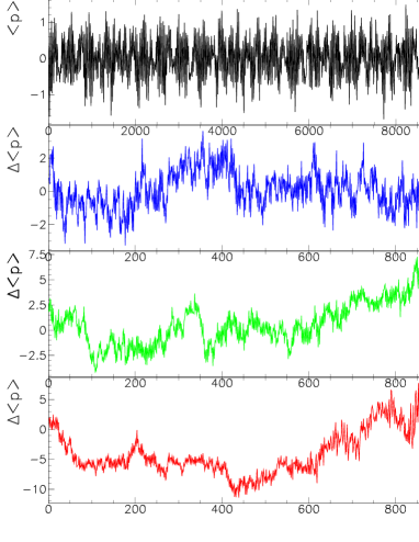
FIG. 14.: (a) Tunnelling oscillations in the non resonant Kicked Rotator; (b),(c),(d) suppression of dynamical tunneling of the first moment $\langle p(t)\rangle$ in the presence of nonlinear perturbation ((b) $u=5$, (c)$u=10$, (d)$u=20$). The difference $\Delta\langle p(t)\rangle$ is plotted. The parameters values are $\tau=1$, $k=4.42,N=128,L=2000$.

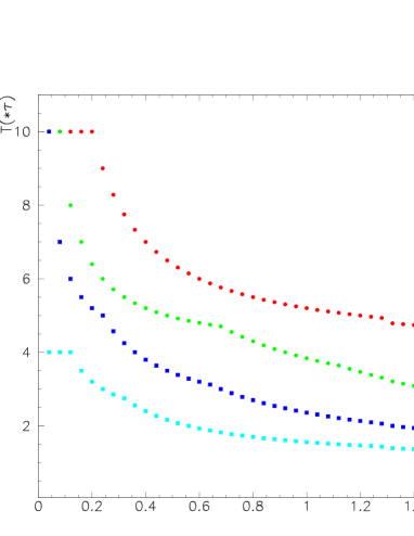
FIG. 15.: Time $T$ at which $|\Delta\langle p(t)\rangle|$ becomes greater than $\Delta$ versus the nonlinear parameter $u$. Each curve correspond to a different values of $\Delta$: $\Delta=0.4,0.2,0.1,0.05$ starting from above.

In accordance with [16], the nonlinear perturbation suppresses localization and give rise to an anomalous diffusion with an exponent approximately equal to $2/5$. In fig.13 a bilogarithmic plot of the time-integrated second moment $P_{int}^{2}(t)=\frac{1}{t}\sum_{t^{\prime}=0}^{t-1}\langle p^{2}(t^{\prime})\rangle$ for $k=2.5$ and for different values of $u$ is shown; the straight line in the figure has a slope of $2/5$.

Tunnelling oscillations of $\langle p(t)\rangle$ for the Kicked Rotator are plotted in fig.14(a). In Fig.14 (b),(c),(d), we show the suppression of tunnelling oscillations of the first moment for different values of the nonlinear parameter (b)$u=5$, (c)$u=10$, (d) $u=20$. The differences $\Delta\langle p(t)\rangle=\langle p(t)\rangle_{u}-\langle p(t)\rangle_{0}$ are plotted.

In Fig.15 the time $T$ at which $|\Delta\langle p(t)\rangle|$ becomes greater that $\Delta$ versus $u$ is plotted. Each curve corresponds to a different values of $\Delta$. Note that the evolution of $\langle p(t)\rangle$ in the kicked rotator is calculated at time intervals equals to $\tau$, therefore the estimate of the time $T$ is less precise than that calculated for the driven pendulum.

IV Conclusions.

We have analyzed different physical systems for which dynamical tunneling occurs: in particular the driven pendulum and the kicked rotator. These systems are relevant for experimental settings recently realized with cold atoms. We have stressed several new features: from the role of how initially quasimomentum states are assembled, to the effect of Gross-Pitaevskii nonlinearities, in particular revealing subtle features happening in the resonant kicked rotator case.

Acknowledgments.

This work was partially supported by EU contract QTRANS network (Quantum Transport on an Atomic Scale) and INFM PA project (Weak Chaos: theory and applications).

$\Delta$	$B$	$A$
0.005	0.0719$\pm$0.0012	0.1547$\pm$0.0096
0.01	0.0836$\pm$0.0012	0.1649$\pm$0.0084
0.02	0.0979$\pm$0.0011	0.1664$\pm$0.0072
0.05	0.1219$\pm$0.0011	0.1908$\pm$0.0059
0.1	0.1456$\pm$0.0010	0.2031$\pm$0.0050
0.2	0.1766$\pm$0.0012	0.2193$\pm$0.0042

TABLE I.: Fitting parameters of $T$.

REFERENCES

- [1] D.A. Steck, W.H. Oskay and M.G. Raizen, Science, Vol.293, 274 (2001).
- [2] R. Balian and C. Bloch, Ann. Phys. (N.Y.), 84, 559 (1974).
- [3] M. Wilkinson, Physica D21, 341 (1986); M. Wilkinson and J.H. Hannay, Physica D27, 201 (1987).
- [4] M.J. Davis and E.J. Heller, J. Chem. Phys.75, 264 (1981).
- [5] S. Tomsovic and D. Ullmo, Phys. Rev. E50, 145 (1994).
- [6] A. Mouchet, C. Miniatura, R. Kaiser, B. Grémaud and D. Delande, Phys.Rev.E, 64, 016221 (2001).
- [7] A. Mouchet and D. Delande, Phys. Rev. E67, 046216 (2003).
- [8] C. Dembowski, H.D. Gräf, A. Heine, R. Hofferbert, H. Rehfeld and A. Richter, Phys. Rev. Lett. 84, 867 (2000).
- [9] W.K. Hensinger, H. Häffuer, A. Browaeys, N.R. Heckenberg, K. Helmerson, C. McKenzie, G.J. Milburn, W.D. Phillips, S.L. Rolston, H. Rubinzlein-Dunlop and B. Upcroft, Nature 412, 52 (2001).
- [10] See, for instance, the rewiew by W. Ketterle at al. in “Bose-Einstein Condensation in Atomic Gases”, edited by M. Inguscio, S. Stringari and C. Wieman (IOS Press, Amsterdam, 1999); E. Cornell at al., ibid.
- [11] See F. Dalfovo, S. Giorgini, L.P. Pitaevskii and S. Stringari, Rev. Mod. Phys. 71, 463 (1999), and referencies therein.
- [12] G.P. Berman, V.Yu. Rubaev and G.M. Zaslavsky, Nonlinearity 4, 543 (1991); F. Borgonovi and L. Rebuzzini, Phys. Rev. E52, 2302 (1995); D. Shepelyansky and C. Sire, Europhys. Lett. 20, 95 (1992).
- [13] S.A. Gardiner, D.Jaksch, R.Dum, J.I. Cirac and P. Zoller, Phys.Rev. A62, 023612 (2000);
- [14] R. Artuso and L. Rebuzzini, Phys.Rev.E 66, 017203 (2002).
- [15] F. Benvenuto, G. Casati, A.S. Pikovsky and D.L. Shepelyansky, Phys.Rev.A, 44, R3423 (1991).
- [16] D.L. Shepelyansky, Phys.Rev.Lett, 70, 1787 (1993).
- [17] D.A. Steck, V. Milner, W.H. Oskay and M.G. Raizen, Phys.Rev.E 62, 3461 (2000).
- [18] G. Casati, B.V. Chirikov, J. Ford and F.M. Izrailev, “Stochastic Behavior in Classical and Quantum Hamiltonian Systems”, Vol.93, (Springer-Verlag, Berlin, 1979).
- [19] N.W. Ashcroft and N.D. Mermin, “Solid State Physics” (Saunders College, Philadelphia, 1976).
- [20] See, for instance, A.D. Bandrauk and H. Shen, J. Chem. Phys. 99, 1185 (1993).
- [21] R. Luter and L.E. Reichl, Phys. Rev A 66, 053615 (2002).
- [22] S. Fishman, I. Guarneri and L. Rebuzzini, J.Stat.Phys 110, 911 (2003).
- [23] B.V. Chirikov, Phys. Rep. 52, 263 (1979).
- [24] A.J. Lichtemberg and M.A. Lieberman, “Regular and Chaotic Dynamics”, (Springer Verlag, NY, 1992)
- [25] S. Benkadda, S. Kassibrakis, R.B. White and G.M. Zaslavsky, Phys.Rev. E55, 4909 (1997).
- [26] G. Casati, B.V. Chirikov, J. Ford and F.M. Izrailev, Lecture Notes in Physics, edited by G. Casati and J.Ford, Stochastic Behaviour in Classical and Quantum Hamiltonian System, Vol.93 (Springer-Verlag, Berlin, 1979).
- [27] F.M. Izrailev and D.L. Shepelyansky, Matematicheskaya Fizica, 43,n.3, 417 (1980).
- [28] F.M. Izrailev, Phys.Rep. 196, 299 (1990).
- [29] G. Casati, R. Graham, I. Guarneri and F.M. Izrailev, Phys.Lett.A, 190, 159 (1994).
- [30] M. Latka, P. Grigolini and B.J. West, Phys.Rev.A, 50, 1071 (1994).
- [31] S.J. Chang and K.J. Shi, Phys.Rev.A, 34, 7 (1986).