On the canonically invariant calculation of Maslov indices

M Pletyukhov¹ and M Brack

Institute for Theoretical Physics, University of Regensburg, D-93040 Regensburg, Germany

¹e-mail: mikhail.pletyukhov@physik.uni-regensburg.de

Abstract

After a short review of various ways to calculate the Maslov index appearing in semiclassical Gutzwiller type trace formulae, we discuss a coordinate-independent and canonically invariant formulation recently proposed by A Sugita (2000, 2001). We give explicit formulae for its ingredients and test them numerically for periodic orbits in several Hamiltonian systems with mixed dynamics. We demonstrate how the Maslov indices and their ingredients can be useful in the classification of periodic orbits in complicated bifurcation scenarios, for instance in a novel sequence of seven orbits born out of a tangent bifurcation in the Hénon-Heiles system.

1 Introduction

The idea of Gutzwiller [1] to express the quantum-mechanical density of states of a Hamiltonian system in terms of its classical periodic orbits and their properties has brought an enormous progress to the field of “quantum chaos” [2]. The trace formula which he derived in 1971 [1] is valid for systems in which all periodic orbits are isolated in phase space. Later versions of trace formulae were formulated for integrable systems [3, 4] and mixed systems with continuous symmetries [3, 5, 6], and very recently also for systems with explicit spin degrees of freedom [7, 8].

An important ingredient in all these trace formulae is, besides the action and stability of a periodic orbit, the so-called Maslov index. It is an invariant property of a periodic orbit which can change only when the orbit undergoes a bifurcation or when a continuous symmetry is broken or restored under the variation of a system parameter (eg energy, deformation or an external field). The calculation of the Maslov index is not always straightforward, in particular for systems with many degrees of freedom or systems which are not of the “kinetic plus potential energy” type. In the standard methods used in the literature [9, 10, 11], the determination of the Maslov index of a stable orbit necessitates the explicit use of an “intrinsic” coordinate system that follows the orbit (as introduced by Gutzwiller [1]), which can be numerically quite cumbersome. Easy-to-use calculational recipes using the method of [11] have been given in the appendix D of [12].

Recently, Sugita [13] has given a formula for the Maslov index which only contains canonically invariant ingredients. However, no practical recipes were given for the explicit calculation of the winding number $m$ [see equation (7) in section 2.2]. Inspired by another recent work on semiclassical trace formulae and Maslov indices [14], we have developed simple calculational recipes for the winding number and the stability angle used in Sugita’s formula [13]. The purpose of the present paper is to implement these recipes for various Hamiltonian systems with mixed dynamics and to test their results towards those obtained with the standard methods [1, 10, 11]. As an outcome, we shall give some empirical rules for the behaviour of some of the ingredients of the Maslov indices at bifurcations and demonstrate that they can be useful for the classification of periodic orbits in connection with complicated bifurcation scenarios.

2 General formalism

2.1 Trace formulae and role of Maslov indices

For isolated orbits, Gutzwiller’s trace formula [1] for the oscillating part of the density of states $g(E)$ reads

$$\delta g(E)=\frac{1}{\pi\hbar}\,\sum_{\mathrm{ppo}}\,T_{\mathrm{ppo}}(E)\,\sum_{r=1}^{\infty}\frac{1}{\sqrt{|\det(M^{r}_{\mathrm{red}}-I)|}}\,\cos\left[\frac{r}{\hbar}\,S_{\mathrm{ppo}}(E)-\frac{\pi}{2}\,\sigma_{r}\right],$$ (1)

where $T_{\mathrm{ppo}}$ and $S_{\mathrm{ppo}}$ are the periods and actions of the primitive periodic orbits (ppo) and $r$ is an index which counts the repetitions of the primitive orbits. $M_{\mathrm{red}}$ is their reduced monodromy matrix – often called stability matrix – and $\sigma_{r}$ is the Maslov index of the repeated orbit (which for stable orbits is not a multiple of that of the primitive orbit). For isolated orbits the Maslov index is always an integer, irrespectively of the dimensionality of the system.

For systems with continuous symmetries, periodic orbits are no longer isolated in phase space but come in degenerate families. The semiclassical trace formulae can still be written in the general form

$$\delta g(E)=\sum_{\mathrm{po}}\,{\cal A}_{\mathrm{po}}(E)\,\cos\left[\frac{1}{\hbar}\,S_{\mathrm{po}}(E)-\frac{\pi}{2}\,\sigma_{\mathrm{po}}\right],$$ (2)

where “po” now refers to all repeated families and isolated orbits. The amplitudes ${\cal A}_{\mathrm{po}}(E)$ depend on the degeneracies of the orbit families, besides their stabilities, and have been given in the literature [3, 5, 6]. The Maslov index $\sigma_{\mathrm{po}}$ of an orbit family can be a half integer. Its determination, especially for families with high degeneracies such as they occur in isotropic harmonic oscillators with SU(N) symmetry, is by no means trivial. Although some hints may be found in [6, 13, 14, 15] there exists, to our knowledge, no simple recipe for their calculation. We shall in the remainder of the present paper restrict ourselves to systems with isolated orbits.

It has been shown [11, 16] that the Maslov index of an isolated orbit is a canonical invariant, independent of the orbit’s intrinsic coordinate system and of the starting point for the calculation of the monodromy matrix. However, the published practical ways for its calculation [1, 10, 11] do make explicit use of the orbit’s intrinsic coordinate system. Furthermore, using the form

$$\sigma_{\rm po}=\mu_{\rm po}+\nu_{\rm po}$$ (3)

given in [11] – whereby the part $\mu_{\rm po}$ is the Morse index appearing in the semiclassical Green’s function and the part $\nu_{\rm po}$ comes from the stationary-phase integrations transverse to the orbit – it has been explicitly demonstrated for an unstable orbit that $\mu$ and $\nu$ alone need not be invariant and may, in fact, depend explicitly on its starting point.

A remark on the name “Maslov index” might be in place here. Originally, the Maslov index was introduced in the framework of the WKB and later the EBK quantization of integrable systems [17, 18, 19]. The quantity $\sigma_{\rm po}$ appearing in the above trace formulae is a different index, although for integrable systems it can be easily related [4, 6] to the Maslov indices of the EBK quantization. In the standard literature on the periodic orbit theory, the name of $\sigma_{\rm po}$ has, however, established itself as “Maslov index” and we want here to adhere to this convention.

The trace formulae (1) and (2) provide an approximative description of the quantum-mechanical density of states in terms of classical periodic orbits and their properties. It is obvious that the Maslov index $\sigma_{\rm po}$ plays a vital role in establishing the correct quantum phase interferences and therefore must be determined correctly.

2.2 Invariant calculation of the Maslov index

All information about the Maslov index of an isolated orbit is contained in its matrizant $M(t)$ describing the time propagation of a small perturbation $\delta q,\delta p$ around the orbit in phase space:

$$\left(\begin{array}[]{c}\delta q(t)\\ \delta p(t)\end{array}\right)\;=\;M(t)\left(\begin{array}[]{c}\delta q(0)\\ \delta p(0)\end{array}\right),$$ (4)

where $q(t)$ and $p(t)$ are $N$-dimensional coordinate and momentum variables. $M(t)$ is obtained by solving the linearized equations of motion of a classical system characterized by its Hamiltonian $H(q,p)$, which leads to the differential equations

$$\frac{\mathrm{d}}{\mathrm{d}t}M(t)=JH^{\prime\prime}(t)M(t),\qquad M(0)=I_{2N}\,,$$ (5)

where

$$J=\left(\begin{array}[]{cc}0&I_{N}\\ \!-I_{N}&0\end{array}\right),\qquad H^{\prime\prime}(t)=\left(\begin{array}[]{c@{\hspace{.1cm}}c}\frac{\partial^{2}H}{\partial q\partial q}\hfil\hskip 2.84544pt&\frac{\partial^{2}H}{\partial q\partial p}\vspace*{0.15cm}\\ \frac{\partial^{2}H}{\partial p\partial q}\hfil\hskip 2.84544pt&\frac{\partial^{2}H}{\partial p\partial p}\end{array}\right).$$ (6)

$J$ is the unit symplectic matrix in the $2N$-dimensional phase space, and $I_{2N}$, $I_{N}$ are the $2N$- and $N$-dimensional unit matrices, respectively. At the time of the orbit’s period $T$, the matrix $M(T)$ is called the monodromy matrix. One can always transform $M(T)$ into block form. One parabolic (2$\times$2) block contains the trivial unit eigenvalues related to energy conservation; the remaining $(2N-2)$-dimensional part of $M(T)$ is called the reduced monodromy matrix $M_{\rm red}$ or stability matrix. $M_{\rm red}$ falls into (inverse) parabolic, elliptic, or (inverse) hyperbolic (2$\times$2) blocks or, for $N>2$ dimensions, loxodromic (4$\times$4) blocks, depending on the stability of the respective orbits.

The amplitude in the Gutzwiller trace formula (1) diverges when $\det(M^{r}_{\mathrm{red}}-I)$ becomes zero. For isolated orbits this happens at bifurcations, where an orbit changes from stable to hyperbolically unstable or vice versa, or when a continuous symmetry is restored under the variation of a system parameter such as energy, deformation or some external field. At such singular points $M^{r}_{\mathrm{red}}$ contains an extra parabolic block. The trace formula (1) then cannot be used and one must resort to uniform approximations [20, 21, 22, 23] which we, however, shall not be concerned with in the present paper. We just mention here that bifurcation and symmetry-restoring points are the only places where a Maslov index is allowed to change. The corresponding rules for bifurcations can be found in [21]; an example for the changes of Maslov indices under symmetry breaking (or restoring) will be mentioned in section 2.3.

Referring to the block form of the stability matrix, Sugita [13] has recently proposed the following general formula for the Maslov index $\sigma_{r}$ in (1) of an isolated periodic orbit:

$$\sigma_{r}=\sum_{i=1}^{n_{{\rm ell}}}\left(1+2\left[\frac{r\chi_{i}}{2\pi}\right]\right)+rn_{{\rm ih}}+2mr\,.$$ (7)

Here $[x]$ denotes the integer part of $x$ (ie the largest integer number $\leq x$), $n_{{\rm ell}}$ is the number of elliptic blocks and $\chi_{i}$ the stability angle of the $i$th elliptic block, $n_{{\rm ih}}$ is the number of inverse-hyperbolic blocks, and $m$ is a winding number. Sugita has also discussed in [13] the relation of the winding number $m$ to the homotopy theory. However, no explicit prescription for the computation of $m$ has been given.

This question has been partially answered in a recent review article on periodic orbit theory [14]. The winding number $m$ has been identified as the Gel’fand-Lidski winding number [24], and it has been explained how to calculate it in principle. Muratore-Ginanneschi [14] has also discussed a relation of $\sigma_{r}$ given by (7) to an index which is known in the mathematical literature after the names of Conley and Zehnder [25], and has provided extensive references on the latter subject. However, in [14] the way of extracting a unique value of the stability angle $\chi_{i}$ from the the eigenvalues $e^{\pm i\chi_{i}}$ of the stability matrix has only been hinted at, and a practical algorithm still remained to be specified. We also want to remark that a representation similar to (7) appears in a mathematical paper [15] where a classification of the admissible normal forms of the elements of Sp(2N) is given.

The goal of the present section is to specify the definitions of $\chi_{i}$ and $m$, in order to make the definition of $\sigma_{r}$ in (7) unique and useful for practical applications. In particular, we are going to establish how the choice of $\chi_{i}$ made in [13] corresponds to the prescription for the calculation of $m$ given in [14].

Following [14], we split $M(t)$ into a product of a periodic and an average part (also called the Floquet decomposition):

$$M(t)=M_{{\rm per}}(t)M_{{\rm av}}(t)$$ (8)

with

$$M_{{\rm av}}(t)=\exp(tK)\,,$$ (9)

where $K$ is a constant matrix. By definition, the periodic part of the matrizant in (8) satisfies the condition $M_{{\rm per}}(t)=M_{{\rm per}}(t+T)$. In particular, $M_{{\rm per}}(0)=M_{{\rm per}}(T)=I_{2N}$. We therefore can specify the constant matrix $K$ by equating

$$M_{{\rm av}}(T)\equiv\exp(TK)=M(T)\,.$$ (10)

Then, we get

$$K=\frac{1}{T}\ln[M(T)]\,.$$ (11)

To take the logarithm on the rhs of (11), we diagonalize $M(T)$, calculate the logarithms of the eigenvalues of $M(T)$, and then return to the initial basis. However, the relation (11) remains symbolic until we adopt a certain phase convention for determining the eigenvalues of $K$.

In the standard definition of the function $\ln(z)$ with $z=|z|e^{i\phi}$, the phase range $\phi\in(-\pi,\pi]$ is chosen, corresponding to the branch cut line being taken along the negative real axis. Let us consider the eigenvalue problem

$$M(T)\,\xi_{i}^{\pm}=e^{\pm i\widetilde{\chi}_{i}}\,\xi_{i}^{\pm}\,,$$ (12)

with $\xi_{i}^{-}=[\xi_{i}^{+}]^{*}$ and

$$\widetilde{\chi}_{i}=-i\ln[e^{+i\widetilde{\chi}_{i}}]\in(0,\pi)\,.$$ (13)

The case $\widetilde{\chi}_{i}=\pi$ will be discussed separately below.

Let us now introduce the symplectic product

$$s_{i}=+[{\rm Re}(\xi_{i}^{+})]^{{\rm T}}J\,{\rm Im}(\xi_{i}^{+})\equiv-[{\rm Re}(\xi_{i}^{-})]^{{\rm T}}J\,{\rm Im}(\xi_{i}^{-})\,,$$ (14)

known as the Krein invariant [19, 26]. With this, we can adopt the following convention for the eigenvalues $\pm i\frac{\chi_{i}}{T}$ of $K$:

$$K\xi_{i}^{\pm}=\pm i\frac{\chi_{i}}{T}\,\xi_{i}^{\pm}\,,$$ (15)

so that

$$\chi_{i} = \widetilde{\chi}_{i}\qquad\quad\,\,{\rm for}\quad s_{i}>0\,,$$

$$\chi_{i} = 2\pi-\widetilde{\chi}_{i}\quad{\rm for}\quad s_{i}<0\,.$$ (16)

These relations fully determine the constant matrix $K$ and specify uniquely the stability angle to be used in the formula (7). In this phase convention, $\chi_{i}$ takes values in the range $(0,2\pi)$.

The case of an inverse parabolic block with $\,e^{\pm i\widetilde{\chi}_{i}}=-1$ is degenerate and requires special consideration. It occurs when $\mathrm{tr}M_{\mathrm{red}}=-2$ and corresponds to the stability changing between elliptic and inverse hyperbolic. In this case we choose the value $\chi_{i}=\pi$ by continuity reasons. The inverse parabolic block should be taken into accout in the formula (7) as a special case of either an inverse hyperbolic or an elliptic block, but not twice – in order to avoid double counting.

The winding number $m$ is an invariant characteristic of $M_{{\rm per}}(t)=M(t)M^{-1}_{{\rm av}}(t)$. To determine it, it is convenient to employ the so-called polar decomposition of the symplectic matrix $M_{\mathrm{per}}$ into a product of an orthogonal matrix $R_{\mathrm{per}}$ and a positive-definite symmetric matrix $W_{\mathrm{per}}$:

$$M_{\mathrm{per}}=R_{\mathrm{per}}\,W_{\mathrm{per}}\,.$$ (17)

In turn, the orthogonal matrix $R_{\mathrm{per}}$ admits the representation

$$R_{\mathrm{per}}=\left(\begin{array}[]{cc}X_{\mathrm{per}}&Y_{\mathrm{per}}\\ -Y_{\mathrm{per}}&X_{\mathrm{per}}\end{array}\right).$$ (18)

Therefore, the winding number $m$ can be defined as

$$m=\varphi(T)-\varphi(0)\,,$$ (19)

where

$$\varphi(t)=\frac{1}{2\pi}\mathrm{Arg}\det\left[X_{{\rm per}}(t)+iY_{{\rm per}}(t)\right].$$ (20)

Since $X_{\mathrm{per}}(t)$ and $Y_{\mathrm{per}}(t)$ are periodic, $m$ is a (positive or negative) integer number.

The winding number (19) has been vastly discussed in the literature, both mathematical and physical (see [14] for extensive references). In particular, we would like to quote here that it has been introduced in [24] for a topological characterization of the structural stability of linear Hamiltonian flow.

The extraction of $R_{{\rm per}}(t)$ from $M_{{\rm per}}(t)$ provides a nice representation of the evolution of $\varphi(t)$, because $\det[X_{{\rm per}}(t)+iY_{{\rm per}}(t)]$ runs around the unit circle. However, the polar decomposition (17) is not essential for the calculation of the winding number $m$, even though the latter is encoded in $R_{\mathrm{per}}(t)$. The same result as in (20) can be also obtained from $\psi(T)-\psi(0)$, where

$$\psi(t)=\frac{1}{2\pi}\mathrm{Arg}\det\left[A_{{\rm per}}(t)+iB_{{\rm per}}(t)\right],$$ (21)

and the matrices $A_{{\rm per}}(t)$ and $B_{{\rm per}}(t)$ are the blocks of

$$M_{{\rm per}}(t)=\left(\begin{array}[]{cc}A_{{\rm per}}(t)&B_{{\rm per}}(t)\\ C_{{\rm per}}(t)&D_{{\rm per}}(t)\end{array}\right).$$ (22)

For a proof and further discussion of this point, see the Appendix A of [27].

Let us now consider the following canonical transformation

$$M(t)=S(t)M_{{\rm av}}(t)S(0)^{-1}\,.$$ (23)

with $S(t)\equiv M_{{\rm per}}(t)$. Since $S(0)=I_{2N}$, this expression is equivalent to (8). The relation between the Maslov indices $\sigma$ of $M(t)$ and $\sigma_{{\rm av}}$ of $M_{{\rm av}}(t)$ for $r=1$ is given by [13]

$$\sigma=\sigma_{{\rm av}}+2m\,.$$ (24)

But the winding number in $\sigma_{{\rm av}}$ equals zero, since $M_{{\rm av}}(t)$ belongs to the same homotopy class as the identity matrix, ie it can be continuously shrunk to the latter. Therefore, in order to determine $\sigma_{{\rm av}}$ we just need to find the number of elliptic and inverse hyperbolic blocks, which can be read off the block form of $M_{{\rm av}}(T)=M(T)$. We remark that neither $\sigma_{{\rm av}}$ nor $m$ depend on the choice of the starting point on the periodic orbit [13], as it must be for canonically invariant quantities.

We note in passing that the Maslov index $\sigma_{r}$ can be identified with the winding number obtained from a polar decomposition of the whole matrizant $M(t)$ [16]. However, that approach also requires some further specifications for stable orbits.

This completes our specification of Sugita’s approach. Before discussing another choice of the phase convention which allows us to make contact with the earlier approach of [11], we will illustrate our method with an analytical example.

2.3 Analytical example: irrational harmonic oscillators

We consider here a simple integrable system with isolated orbits, for which all the above quantitites can be evaluated analytically. This is the two-dimensional anisotropic harmonic oscillator

$$H=\frac{1}{2}\,(p_{x}^{2}+p_{y}^{2})+\frac{1}{2}\,(\omega_{x}^{2}x^{2}+\omega_{y}^{2}y^{2})=\frac{\omega_{x}}{2}\,(P_{x}^{2}+Q_{x}^{2})+\frac{\omega_{y}}{2}\,(P_{y}^{2}+Q_{y}^{2})\,,$$ (25)

where $Q_{x}=x\sqrt{\omega_{x}}$, $Q_{y}=y\sqrt{\omega_{y}}$ and $P_{x}=p_{x}/\!\sqrt{\omega_{x}}$, $P_{y}=p_{y}/\!\sqrt{\omega_{y}}$. We assume that the frequencies $\omega_{x}$ and $\omega_{y}$ are incommensurate, so that the only periodic orbits are librations along the $x$ and $y$ axes; they are isolated and stable. For the orbit along the $x$ axis, the period is $T_{x}=2\pi/\omega_{x}$, and the monodromy matrix and its periodic and average parts are, respectively, given by (cf [12, 28])

$$M_{x}(t) = \left(\begin{array}[]{cccc}\cos(\omega_{x}t)&0&\sin(\omega_{x}t)&0\\ 0&\cos(\omega_{y}t)&0&\sin(\omega_{y}t)\\ -\sin(\omega_{x}t)&0&\cos(\omega_{x}t)&0\\ 0&-\sin(\omega_{y}t)&0&\cos(\omega_{y}t)\end{array}\right),$$ (30)

$$M_{x,{\rm per}}(t) = \left(\begin{array}[]{cccc}\cos(\omega_{x}t)&0&\sin(\omega_{x}t)&0\\ 0&\cos(\Delta\omega_{y}\,t)&0&\sin(\Delta\,\omega_{y}t)\\ -\sin(\omega_{x}t)&0&\cos(\omega_{x}t)&0\\ 0&-\sin(\Delta\omega_{y}\,t)&0&\cos(\Delta\,\omega_{y}t)\end{array}\right),$$ (35)

$$M_{x,{\rm av}}(t) = \left(\begin{array}[]{cccc}1&0&0&0\\ 0&\cos(\bar{\omega}_{y}t)&0&\sin(\bar{\omega}_{y}t)\\ 0&0&1&0\\ 0&-\sin(\bar{\omega}_{y}t)&0&\cos(\bar{\omega}_{y}t)\end{array}\right),$$ (40)

where

$$\bar{\omega}_{y}=\omega_{y}-\omega_{x}\left[\frac{\omega_{y}}{\omega_{x}}\right],\quad\Delta\omega_{y}=\omega_{y}-\bar{\omega}_{y}=\omega_{x}\left[\frac{\omega_{y}}{\omega_{x}}\right].$$ (41)

In order to calculate the winding number $m_{x}$, we consider

$$\mathrm{Arg}\det\left[X_{x,{\rm per}}(t)+iY_{x,{\rm per}}(t)\right]=(\omega_{x}+\Delta\omega_{y})\,t\,.$$ (42)

Then we obtain easily

$$m_{x}=\frac{\omega_{x}+\Delta\omega_{y}}{\omega_{x}}=1+\left[\frac{\omega_{y}}{\omega_{x}}\right].$$ (43)

Next we calculate $\chi_{x}/2\pi$:

$$\frac{\chi_{x}}{2\pi}=\frac{\bar{\omega}_{y}}{\omega_{x}}=\frac{\omega_{y}}{\omega_{x}}-\left[\frac{\omega_{y}}{\omega_{x}}\right].$$ (44)

Finally, we obtain the Maslov index for the $r$th repetition to be

$$\sigma_{x,r}=1+2\left[\frac{r\chi_{x}}{2\pi}\right]+2rm_{x}=1+2\left[r\frac{\omega_{y}}{\omega_{x}}-r\left[\frac{\omega_{y}}{\omega_{x}}\right]\right]+2r\left(1+\left[\frac{\omega_{y}}{\omega_{x}}\right]\right)=1+2r+2\left[r\frac{\omega_{y}}{\omega_{x}}\right].$$ (45)

This result agrees with that obtained in [28] using the method of [11].

A note about the isotropic harmonic oscillator with $\omega_{x}=\omega_{y}=\omega$ may be of some interest here. The periodic orbits in this system, due to its SU(2) symmetry, are not isolated but form families of two-fold degenerate orbits. (The same is true for arbitrary rational axis ratios $\omega_{x}:\omega_{y}=n:p$ with integer $n,p$ for which the orbits are Lissajous figures.) As mentioned in the introduction, we lack a general prescription for the calculation of the Maslov index of these families. However, the semiclassical trace formulae of isotropic harmonic oscillators can be obtained by other means and are found to be quantum-mechanically exact [28]. In two dimensions, the trace formula reads

$$g(E)=\frac{E}{(\hbar\omega)^{2}}\left\{1+2\sum_{r=1}^{\infty}\cos\left(r\frac{2\pi E}{\hbar\omega}\right)\right\},$$ (46)

which supports a Maslov index $\sigma_{r}=0$ (mod 4). Indeed, with our above results we find $m=2$ from (43) and $\chi=0$ from (44), leading to $\sigma_{r}^{(0)}=4r$ which is equivalent to 0 (mod 4). The reason for our identifying this Maslov index for the isotropic harmonic oscillator here is that in the context of perturbation theory, trace formulae for slightly perturbed harmonic oscillators have been developed [29, 30] in which the Maslov indices of the perturbed isolated orbits are obtained analytically, once the value $\sigma_{r}^{(0)}$ for the unperturbed families is known. For instance, in the Hénon-Heiles system discussed later in section 3.2, the unperturbed families break up into three isolated orbits A, B and C as soon as the nonlinearity is turned on [$\varepsilon>0$ in (56)]. The changes in their Maslov indices with respect to $\sigma_{r}^{(0)}$ were found analytically [23] to be $\Delta\sigma_{A}=+1$, $\Delta\sigma_{B}=0$ and $\Delta\sigma_{C}=-1$. Indeed, the numerical methods for the isolated orbits yield $\sigma_{A}=5$, $\sigma_{B}=4$ and $\sigma_{C}=3$, both using the method of [11] (see [31]) and with our present method (see table 2 below).

A straightforward generalization for the $N$-dimensional harmonic oscillator with irrational frequency ratios $\omega_{i}/\omega_{j}$ ($i,j=1,2,\dots,N$) yields the Maslov index for the orbit along the $j$ axis

$$\sigma^{(N)}_{j,r}=(N-1)+2r+2\sum_{{i=1}\atop{i\neq j}}^{N}\left[r\frac{\omega_{i}}{\omega_{j}}\right].$$ (47)

2.4 Alternative prescription and relation to earlier approaches

In this section we introduce another prescription for calculating the quantitities $\chi_{i}$ and $m$ appearing in [13]. It is based on the alternative Floquet decomposition

$$M(t)=\widetilde{M}_{{\rm per}}(t)\,\widetilde{M}_{{\rm av}}(t)\equiv\widetilde{M}_{{\rm per}}(t)\,\exp(t\widetilde{K})\,,$$ (48)

specified by a constant matrix $\widetilde{K}$ such that

$$\widetilde{K}\xi_{i}^{\pm}=\pm i\frac{\widetilde{\chi}_{i}}{T}\,\xi_{i}^{\pm}\,.$$ (49)

This actually represents another convention for the choice of the stability angle. The formula for the Maslov index is then modified to

$$\sigma_{r}=\sum_{i=1}^{n_{{\rm ell}}}\left(1+2\left[\mathrm{sign}(s_{i})\frac{r\widetilde{\chi}_{i}}{2\pi}\right]\right)+rn_{{\rm ih}}+2\,\widetilde{m}r\,.$$ (50)

If $s_{i}>0$ for all $i$, we have $\widetilde{K}=K$ and $\widetilde{\chi}_{i}=\chi_{i}$, as well as $\widetilde{m}=m$. Then, there is no difference between (50) and (7). If $s_{i}<0$ for some $i$, we can make the transformation

$$2\left[-\frac{r\tilde{\chi}_{i}}{2\pi}\right]=-2r+2\left[\frac{r(2\pi-\tilde{\chi}_{i})}{2\pi}\right]=-2r+2\left[\frac{r\chi_{i}}{2\pi}\right].$$ (51)

Correspondingly, the winding number $m$ of $M_{{\rm per}}(t)$ changes to $\widetilde{m}$, which is the winding number of $\widetilde{M}_{{\rm per}}(t)$, such that

$$2\widetilde{m}r=2mr+2r\,.$$ (52)

Summing up (51) and (52), we see that the $\sigma_{r}$ in both (50) and (7) coincide. Thus, the equivalence of both representations is established. We also note that, in general, the difference $(\widetilde{m}-m)$ equals to the winding number of $e^{t(K-\widetilde{K})}$, which is the number of elliptic blocks of $K$ (or $\widetilde{K}$) with negative values of $s_{i}$.

The sign of $s_{i}$ may change from positive to negative (or vice versa) away from bifurcation or symmetry restoring points. As a consequence, $\widetilde{m}$ changes its value by $+1$ or $-1$, but such as to conserve the total Maslov index. In two-dimensional systems, we have found this to happen when the stability discriminant $2-{\rm det}(M_{\rm red}-I_{2})={\rm tr}M_{\rm red}$ crosses or touches the line tr$M_{\rm red}=-2$. The prescription for $\widetilde{K}$ based on (49) is not relevant from the point of view of a canonically invariant formulation, but such a representation often appears to be more convenient in numerical computations. It reveals itself useful, in fact, to establish some relations to the approach of Creagh, Robbins and Littlejohn [11] (see also [16] and Appendix D in [12]). As mentioned already above, these authors have written the Maslov index as a sum (3) of two contributions, which for stable orbits must be calculated separately. For stable orbits, $\mu$ and $\nu$ are invariants in the sense that they do not depend on the starting point of the orbit, but they may change their values away from bifurcations or symmetry restoring points, exactly as it happens for $\widetilde{m}$. We note that for a two-dimensional system, $\nu$ is given [11] by the upper right element $b$ of the stability matrix

$$M_{red}=\left(\begin{array}[]{cc}a&b\\ c&d\end{array}\right)$$ (53)

and can be calculated as

$$b=\frac{\partial r_{\perp}(T)}{\partial p_{\perp}(0)}\,,$$ (54)

where $p_{\perp}(t)$ and $r_{\perp}(t)$ are the momentum and coordinate, respectively, transverse to the orbit. This relation actually demonstrates the necessity of knowing the orbit’s intrinsic coordinate system for the calculation of $b$ and hence of $\nu$.

We conclude this section by a number of rules for the Maslov indices for two-dimensional Hamiltonian systems that are useful for the classification of periodic orbits, in particular in connection with complicated bifurcation scenarios such as will be discussed in our applications in section 3. The rule 1 is rigorous and follows directly from the formulae (7) and (50), whereas the rules 2 – 4 are empirical, being based on numerical experience. They will be illustrated in the examples given in the next section.

• In two-dimensional systems, the Maslov index $\sigma_{r}$ is always even for hyperbolically unstable orbits and odd for stable and inverse-hyperbolically unstable orbits.

• For stable orbits, sign$(s)=\,$ sign$(b)$. This means that ${\widetilde{\sigma}}_{\rm av}$ is always negative when $\nu=0$ and positive when $\nu=1$.

• The values of sign$(s)$ of two stable orbits involved in the same bifurcation are identical.

• All orbits involved in a bifurcation locally have the same winding numbers $\widetilde{m}$.

These rules are consistent with the fact that Maslov indices of isolated orbits can only change at bifurcations and in symmetry-restoring limits. The changes at bifurcations are given in the papers of Sieber and Schomerus [21] and were found to be correctly reproduced by the present method in all cases.

3 Numerical applications

In this section, we shall apply our method to some systems with mixed classical dynamics. We first discuss two textbook systems, the homogeneous two-dimensional quartic oscillator and the famous Hénon-Heiles system. They both have Hamiltonians of the form $H=p^{2}\!/2+V(q)$ and have been investigated numerous times in the framework of periodic orbit theory using the previous methods [10] and [11] for the calculation of the Maslov indices. In the next two examples we shall study systems with spin degrees of freedom, for which a simple separation into kinetic and potential energy is not possible and the previous methods are not straightforwardly applied.

3.1 The quartic oscillator

As a typical system which exhibits the transition from integrable regular to almost completely chaotic motion, we study the quartic oscillator Hamiltonian

$$H=\frac{1}{2}\,(p_{x}^{2}+p_{y}^{2})+\frac{1}{4}\,(x^{4}+y^{4})+\frac{\alpha}{2}\,x^{2}y^{2}\,.$$ (55)

It is homogeneous in coordinates and momenta, so that the energy can be scaled away. The chaoticity parameter is $\alpha$. For $\alpha=0$, 1 and 3, the system is integrable and in the limits $\alpha\rightarrow-1$ and $\alpha\rightarrow\infty$ it becomes nearly chaotic [32]. The stability of the linear orbit running along either of the axes, which we here denote by A, is known analytically [33]. The trace of its stability matrix is given by ${\rm tr}\,M_{\rm red}=4\,\cos(\pi\sqrt{1+8\alpha}/2)+2$. Isochronous bifurcations of the primitive A orbit, which are of pitchfork type, occur when ${\rm tr}\,M_{\rm red}$ takes the value +2 which occurs at the values $\alpha_{n}=\frac{1}{2}\,n\,(n+1)$ with $n=0,3,4,5,\dots$ Period-doubling bifurcations of island-chain type occur at the values $\alpha_{p}=2p\,(p+1)+3/8$ with $p=0,1,2,\dots$ These bifurcations of the A orbit and the analytical properties of the period-one and period-two orbits created at the bifurcations have been discussed in [34] and [35]. As an example for our present evaluation of the winding number $m$, we shown in the left part of figure 1 the function $\varphi(t)$ defined in (20), obtained here for the stable orbit L₇ born at the bifurcation of the A orbit at $\alpha=15$. It yields $m=3$. Since $s>0$ in this case, $\varphi(t)$ is identical to $\widetilde{\varphi}(t)$. The Maslov index becomes $\sigma_{1}=7$, in agreement with the value obtained in [34] using the formalism of [11]. In the right part of figure 1 we show the shape of the L₇ orbit in the $(x,y)$ plane.

Figure 1: Properties of the the L₇ orbit in the quartic oscillator Hamiltonian (55) at $\alpha=16.8$. Left panel: phase function $\varphi(t)$ (20) giving $m=3$; right panel: shape of the L₇ orbit in the $(x,y)$ plane.

In [36], the scaling behaviour of the fix points corresponding to period-four orbits created at bifurcations of the fourth repetition of the A orbit (denoted here by A⁴) have been discussed. To illustrate this scenario, we show in figure 2 the stability discriminant ${\rm tr}\,M_{\rm red}$ of the period-four orbits involved in an island-chain bifurcation of the A⁴ orbit, which occurs at $\alpha=5.4305556$, and in the succeeding pitchfork bifurcations of the P₂₁ and P${}^{\prime}_{21}$ orbits. The subscripts of the orbit names indicate their Maslov indices as obtained using the formulae of [11]. (Not shown are the orbits created at the bifurcations of A⁴ occurring at $\alpha=4.375$ and at $\alpha=6$.)

Figure 2: Stability discriminant ${\rm tr}\,M_{\rm red}$ of the period-four orbits in the quartic oscillator (55) involved in an island-chain bifurcation of the A${}^{4}_{21}$ orbit occurring at $\alpha=5.4305556$ and in the succeeding pitchfork bifurcations of the P₂₁ and P${}^{\prime}_{21}$ orbits.

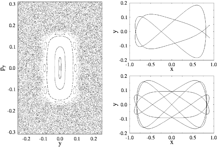
Figure 3: Poincaré surface of section $(y,p_{y})$, shown in the left panel, taken at $x=0$ in the quartic oscillator (55) at $\alpha$=6.0. The fix point in the central stability island corresponds to the A orbit, and the chain of eight unstable and stable fix points correspond to the two pairs of period-four orbits F₂₂ and P₂₁ with shapes shown in the upper and lower right panels, respectively.

In figure 3 we show on the left side a Poincaré surface of section $(y,p_{y})$, taken for $x=0$ at $\alpha=6.0$. The fix point in the central stability island corresponds to the A orbit and its repetitions. The KAM chain of eight unstable and stable fix points, which form the boundary of the stability island towards the chaotic sea, correspond to the two pairs of period-four orbits F₂₂ and P₂₁ whose $(x,y)$ shapes are shown in the upper and lower right panels of figure 3, respectively. These are the fix points whose scaling with $\alpha$ was studied in [36].

Table 1 shows the stabilities, Maslov indices and their ingredients of the above period-four orbits in the quartic oscillator. We give the intervals $(\alpha_{min},\alpha_{max})$ in which the orbits are stable (ell) with a fixed sign of $s$, hyperbolically (hyp) unstable, or inverse-hyperbolically (i-hyp) unstable. Values of $(\alpha_{min}$ and $\alpha_{max})$ marked by an asterisk (*) denote bifurcation points for the orbits listed in the corresponding rows. Note that the values of $\mu$ and $\nu$ are not unique for unstable orbits; they may depend on the starting point along the orbit chosen for their calculation, but such that $\sigma=\mu+\nu$ is invariant [11]. For stable orbits, they are constant in each of the given regions and related to $2\widetilde{m}$ and $\widetilde{\sigma}_{\mathrm{av}}$ as discussed in section 2.4. Our results show the consistent agreement between the definitions of the Maslov index by Creagh et al [11] and by Sugita [13]. They also illustrate the empirical rules given at the end of section 2.4.

orbit	$\alpha_{min}$	$\alpha_{max}$	stab	$m$	$\sigma_{\mathrm{av}}$	$\widetilde{m}$	$\widetilde{\sigma}_{\mathrm{av}}$	$\sigma$	$\mu$	$\nu$
A${}^{4}_{21}$	4.375*	4.913	ell	10	1	10	+1	21	20	1
A${}^{4}_{21}$	4.913	5.431*	ell	10	1	11	$-1$	21	21	0
A${}^{4}_{23}$	5.431*	5.837	ell	11	1	11	+1	23	22	1
A${}^{4}_{23}$	5.837	6.0*	ell	11	1	12	$-1$	23	23	0
A${}^{4}_{24}$	6.0*	10.0*	hyp	12	0	12	0	24	23/24	1/ 0
F22	5.431*	$\infty$	hyp	11	0	11	0	22	21/22	1/ 0
P21	5.431*	6.118	ell	10	1	11	$-1$	21	21	0
P21	6.118	6.262	ell	10	1	10	+1	21	20	1
P20	6.262	$\infty$	hyp	10	0	10	0	20	19/20	1/ 0
P${}^{\prime}_{21}$	6.262	6.341	ell	10	1	10	+1	21	20	1
P${}^{\prime}_{21}$	6.341	6.383	i-hyp	10	1	10	+1	21	20/21	1/ 0
P${}^{\prime}_{21}$	6.383	6.412*	ell	10	1	11	$-1$	21	21	0
P${}^{\prime}_{22}$	6.412*	$\infty$	hyp	11	0	11	0	22	21/22	1/ 0
P${}^{\prime\prime}_{21}$	6.412*	6.422	ell	10	1	11	$-1$	21	21	0
P${}^{\prime\prime}_{21}$	6.422	$\infty$	i-hyp	10	1	10	+1	21	20/21	1/ 0

Table 1:   Stabilities, Maslov indices and related properties of the orbits in the quartic oscillator whose stability discriminants ${\rm tr}\,M_{\rm red}$ are shown in figure 2. ’ell’, ’hyp’ and ’i-hyp’ denote elliptic (stable), hyperbolic and inverse-hyperbolic (unstable) orbits, respectively. Values of $\alpha_{min}$ or $\alpha_{max}$ marked by an asterisk (*) denote bifurcation points for the orbits given in the corresponding row. For unstable orbits, the decomposition of $\sigma=\mu+\nu$ is not unique.

3.2 The Hénon-Heiles system

Another famous system with mixed classical dynamics is given by the Hénon-Heiles Hamiltonian [37]

$$H=\frac{1}{2}\,(p_{x}^{2}+p_{y}^{2})+\frac{1}{2}\,(x^{2}+y^{2})+\varepsilon\,(x^{2}y-\frac{1}{3}\,y^{3})\,,$$ (56)

where $\epsilon$ regulates the chaoticity of the system. The potential in (56) has three saddle points at the energy $E^{*}=1/6\,\varepsilon^{2}$, over which a particle can escape if $E>E^{*}$. The classical dynamics depend only on the scaled energy $e=E/E^{*}=6\,\varepsilon^{2}E$; in this variable the saddles are at $e=1$. Along the symmetry lines passing through the saddles, one of them being the $y$ axis, there are librating orbits (denoted here again by A) whose stability oscillates infinitely many times as the energy approaches the critical value $e=1$, giving rise to an infinite cascade of isochronous pitchfork bifurcations. The scaled bifurcation energies $e_{n}$ ($n=1,2,\dots,\infty$) form a sequence that cumulates at $e_{\infty}=1$ in a Feigenbaum-like fashion; the orbits born at the bifurcations exhibit self-similarity with analytically known scaling constants [38].

At each successive bifurcation $e_{n}$, the A orbit increases its Maslov index by one unit. The orbits born at the bifurcations are alternatingly stable rotations R_σ and unstable librations L_σ; they can be uniquely classified by their increasing Maslov indices: R₅, L₆, R₇, L₈, etc, according to the rules given at the end of section 2.4 (cf also [34, 38]). Besides the A orbit, the system possesses a curved librating orbit B which is unstable at all energies, and a rotating orbit C which is stable up to $e=0.8919$ where it turns inverse hyperbolically unstable. Its

orbit	$e_{min}$	$e_{max}$	stab	$m$	$\sigma_{\mathrm{av}}$	$\widetilde{m}$	$\widetilde{\sigma}_{\mathrm{av}}$	$\sigma$	$\mu$	$\nu$
A5	0.0	0.8117	ell	2	1	2	+1	5	4	1
A5	0.8117	0.9152	i-hyp	2	1	2	+1	5	4/5	1/0
A5	0.9152	0.9693*	ell	2	1	3	$-1$	5	5	0
A6	0.9693*	0.9867*	hyp	3	0	3	0	6	5/6	1/0
R5	0.9693*	0.9895	ell	2	1	3	$-1$	5	5	0
R5	0.9895	$\infty$	i-hyp	2	1	2	+1	5	4/5	1/0
A7	0.9867*	0.9950	ell	3	1	3	+1	7	6	1
L6	0.9867*	$\infty$	hyp	3	0	3	0	6	5/6	1/0
A7	0.9950	0.9978	i-hyp	3	1	3	+1	7	6/7	1/0
A7	0.9978	0.9992*	ell	3	1	4	$-1$	7	7	0
A8	0.9992*	0.9996*	hyp	4	0	4	0	8	7/8	1/0
R7	0.9992*	0.99948	ell	3	1	4	$-1$	7	7	0
R7	0.99948	$\infty$	i-hyp	3	1	3	+1	7	6/7	1/0
B4	0.0	$\infty$	hyp	2	0	2	0	4	3/4	1/0
C3	0.0	0.8921	ell	1	1	2	$-1$	3	3	0
C3	0.8921	$\infty$	i-hyp	1	1	1	+1	3	2/3	1/0
C${}^{2}_{7}$	0.0	0.6146	ell	3	1	4	$-1$	7	7	0
C${}^{2}_{7}$	0.6146	0.8921*	ell	3	1	3	+1	7	6	1
C${}^{2}_{6}$	0.8921*	$\infty$	hyp	3	0	3	0	6	5/6	1/0
D7	0.8921*	1.013	ell	3	1	3	+1	7	6	1
D7	1.013	1.180*	ell	3	1	4	$-1$	7	7	0
D9	1.180*	1.2375	ell	4	1	4	+1	9	8	1
D9	1.2375	$\infty$	i-hyp	4	1	4	+1	9	8/9	1/0

Table 2: Shortest period-one and period-two orbits in the Hénon-Heiles system, their stabilities, Maslov indices and related properties. Notation as in table 1. $e=E/E^{*}$ is the scaled energy; its values denoted by asterisks (*) are bifurcation energies $e_{n}$.

second repetition bifurcates at this energy, giving birth to an orbit D that stays stable up to $e=1.2375$ where it becomes inverse hyperbolically unstable. We have calculated the Maslov index of all these orbits using the formulae given above and verified that they agree with the values obtained in [23, 31, 38] using the method of [11] and in [34] using the method of [10]. The results are given in table 2, again in energy intervals of constant $\widetilde{\sigma}_{\mathrm{av}}$, $\mu$ and $\nu$.

Although tangent bifurcations are known to occur generically in chaotic and mixed-dynamical systems, to our knowledge no such bifurcation has been reported so far in the Hénon-Heiles system. In [34, 38] we have wrongly surmised that all its periodic orbits existing below the barrier energy $e=1$ are derivatives of the generic orbits A, B, C (and their repetitions) through their bifurcations. This was not correct, as we can demonstrate in the following two figures. Here we present a sequence of “spider”-like orbits that are born out of a tangent bifurcation occurring at the scaled energy $e=0.988249$. Their stability discriminants tr$M_{\rm red}$ are shown in figure 4, and their six genuine shapes in the $(y,x)$ plane in figure 5. The generic pair of a orbits, born with Maslov indices 22 and 23, keeps its shape through three successive pitchfork bifurcations at which the orbits c, b and a’ are born; these five orbits remain hyperbolically unstable at all energies $e\,\hbox{\kern 1.00006pt\lower 2.58334pt\hbox{$\sim$} \kern-11.19997pt\raise 2.58334pt\hbox{$>$} }1.016$. The latter two bifurcate again, giving birth

Figure 4: Stability discriminants tr$M_{\rm red}$ of the sequence of “spider” orbits in the Hénon-Heiles potential born out of a tangent bifurcation at the scaled energy $e=0.988249$. The numbers give their Maslov indices $\sigma$ in the respective stability intervals; the letters refer to the six orbit types whose shapes are shown in figure 5; the horizontal dotted lines correspond to tr$M_{\rm red}=\pm 2$.

to the orbits c’ and a” which remain inverse-hyperbolically unstable at all energies $e\,\hbox{\kern 1.00006pt\lower 2.58334pt\hbox{$\sim$} \kern-11.19997pt\raise 2.58334pt\hbox{$>$} }1.016$. Note that the three orbits a, b, c are reflection-symmetric around the symmetry axes (shown by the dotted lines in figure 5) containing the A orbits, whereas the others are not. The Maslov indices, which fulfill again the rules of section 2.4, have been obtained with our present method. We found, in fact, that the earlier methods of [10] and [11] could not be applied safely here: the use of the intrinsic coordinate systems of these complicated orbits is numerically not always stable enough to yield unique results. This actually demonstrates an advantage of the present method which works reliably for not too unstable orbits ($|$tr$M_{\rm red}|\,\hbox{\kern 1.00006pt\lower 2.58334pt\hbox{$\sim$} \kern-11.19997pt\raise 2.58334pt\hbox{$<$} }40$).

Figure 5: Shapes of the “spider” sequence of periodic orbits in the Hénon-Heiles potential.

3.3 A spin-boson system

We consider a spin-boson system defined by the quantum Hamiltonian

$$\hat{H}=\omega_{b}\,\hat{a}^{{\dagger}}\hat{a}+\omega_{s}\,\hat{s}_{3}+\kappa\,(\hat{a}^{{\dagger}}+\hat{a})(\hat{s}_{+}+\hat{s}_{-})\,,\qquad\qquad{\hat{s}}_{\pm}=\hat{s}_{1}\pm i\hat{s}_{2}\,,$$ (57)

where $\hat{s}_{\alpha}=\frac{1}{2}\sigma_{\alpha}\,\,(\alpha=1,2,3)$ are the usual spin operators for $s=\frac{1}{2}$ particles ($\hbar=1$). This model has a broad range of applications in atomic, molecular and solid-state physics and in quantum optics. In the different fields the Hamiltonian (57) bears different names, among them “Rabi Hamiltonian” and “molecular polaron model” (see [39] for a review and further references).

In order to treat this system (semi-)classically, we have to define a phase-space symbol for the Hamiltonian (57). To this purpose we introduce the bosonic operators $\hat{a}=(\hat{Q}_{b}+i\hat{P}_{b})/\sqrt{2}$, $\hat{a}^{{\dagger}}=(\hat{Q}_{b}-i\hat{P}_{b})/\sqrt{2}$ and take their Wigner transforms to define the canonical bosonic variables $(Q_{b},P_{b})$. For the spin variables $n_{\alpha}$ we use the spin coherent-state symbols of the spin operators $\hat{s}_{\alpha}$, divided by the value of spin $s$ (see eg [8]). This leads to the following symbol of the Hamiltonian (57)

$$H=\frac{\omega_{b}}{2}\,(P_{b}^{2}+Q_{b}^{2}-1)+\frac{\omega_{s}}{2}\,n_{3}+\sqrt{2}\kappa\,Q_{b}\,n_{1}\,.$$ (58)

The classical equations of motion read

$$\dot{Q}_{b} = \omega_{b}P_{b}\,,\qquad\dot{P}_{b}\;=\;-\omega_{b}Q_{b}-\sqrt{2}\kappa n_{1}\,,$$ (59)

$$\dot{n}_{1} = -\omega_{s}n_{2}\,,\quad\;\;\dot{n}_{2}\;=\;\omega_{s}n_{1}-\kappa Q_{b}n_{3}/\sqrt{2}\,,\quad\;\;\dot{n}_{3}\;=\;\kappa Q_{b}n_{2}/\sqrt{2}\,,$$ (60)

with the constraint $n_{1}^{2}+n_{2}^{2}+n_{3}^{2}=1$.

We can now introduce the Darboux coordinates $(Q_{s},P_{s})$ by making a stereographic projection from the North Pole of the unit ${\bf n}$-sphere onto the complex plane and then contracting the plane to a disc with radius $\sqrt{2}$:

$$n_{1}=P_{s}\sqrt{2-P_{s}^{2}-Q_{s}^{2}}\,,\qquad n_{2}=Q_{s}\sqrt{2-P_{s}^{2}-Q_{s}^{2}}\,,\qquad n_{3}=P_{s}^{2}+Q_{s}^{2}-1\,.$$ (61)

Under this mapping, the North Pole is projected onto the boundary of the disc $P_{s}^{2}+Q_{s}^{2}=2$, and the South Pole is projected into the centre of the disc. The Hamiltonian then has the form

$$H=\frac{\omega_{b}}{2}\,(P_{b}^{2}+Q_{b}^{2}-1)+\frac{\omega_{s}}{2}\,(P_{s}^{2}+Q_{s}^{2}-1)+\kappa\,Q_{b}P_{s}\sqrt{2(2-P_{s}^{2}-Q_{s}^{2})}\,.$$ (62)

This is a two-dimensional harmonic oscillator, perturbed by the nonlinear term proportional to $\kappa$. The representation (61) is convenient because the equations of motion (59), (60) for both boson and spin variables can now be written in a canonical Hamiltonian form:

$$\dot{Q}_{a}=\frac{\partial H}{\partial P_{a}},\qquad\dot{P}_{a}=-\frac{\partial H}{\partial Q_{a}},\qquad\qquad(a=b,s)$$ (63)

and the equation for the matrizant $M(t)$ is easily found.

However, as soon as we cross the North Pole on the ${\bf n}$-sphere, the equations (63) become singular, and one has to switch to the alternative representation

$$n_{1}=P_{s}\sqrt{2-P_{s}^{2}-Q_{s}^{2}}\,,\qquad n_{2}=-Q_{s}\sqrt{2-P_{s}^{2}-Q_{s}^{2}}\,,\qquad n_{3}=1-P_{s}^{2}-Q_{s}^{2}\,,$$ (64)

which corresponds to the projection from the South Pole.

The ($Q_{b}$, $P_{b}$) sections of the periodic orbits in this system are similar to those of the orbits in the unperturbed harmonic oscillator ($\kappa=0$), while the spin components $n_{\alpha}$ on the sphere – or, correspondingly, on the ($Q_{s}$, $P_{s}$) disc – evolve substantially with increasing coupling constant $\kappa$. For small $\kappa$, the two periodic orbits R₃ and R₅ originate from the South and the North Pole, respectively (figure 7). In the ($Q_{b},Q_{s}$) space they are simple rotations with Maslov indices 3 and 5, respectively (figure 6), becoming more and more distorted with increasing $\kappa$. At larger values of $\kappa$ they undergo pitchfork bifurcations (see figure 9), giving birth to the orbits P₃ and Q₅, respectively. The ($Q_{b},Q_{s}$) shapes of the four orbits R₂, R₆, P₃ and Q₅ at $\kappa=0.27$ are shown in figure 8. (The subscripts in R_σ and Q_σ denote again the Maslov indices of the respective orbits.)

We note that in the limit $\kappa\to 0$ the Maslov index of the orbit R₃ coincides with the Maslov index ($\sigma=3$) of the shortest isolated orbit in the unperturbed harmonic oscillator (45) with the frequency ratio $\omega_{s}:\omega_{b}=0.6$. The orbit R₅ is ill-defined in the representation (61) in this limit, and we have to switch to (64) instead. For the Hamiltonian (58), this is equivalent to changing $\omega_{s}\to-\omega_{s}$. Then, the formula (45) yields $\sigma=1$ which is equal to 5 (mod 4). The difference can be associated with the Maslov index of the matrix which transforms the matrizant in the representation (61) to the matrizant in the representation (64), even though this matrix is not defined at $\kappa=0$.

Figure 6: ($Q_{b},Q_{s}$) shapes of orbits R₃ (solid line) and R₅ (dashed line) in the spin-boson system (62) at $\kappa=0.05$. Other parameters as in figure 8.

Figure 7: Spin components $n_{\alpha}$ of the orbits R₃ and R₅ in the spin-boson system (62) at $\kappa=0.05$. Other parameters as in figure 8.

Figure 8: Shapes $Q_{s}$ versus $Q_{b}$ of the four orbits R₂, R₆, P₃ and Q₅ (from left to right) in the spin-boson model (62) at $\kappa=0.27$. Other parameter values: $\omega_{b}=1.0$, $\omega_{s}=0.6$, $E=4.0$.

Figure 9: Stability discriminants of the shortest periodic orbits in the spin-boson Hamiltonian (62) with versus $\kappa$. Other parameters as in figure 8. The subscripts denote the Maslov indices.

The bifurcation scenario is shown in figure 9, where we plot the discriminants tr$M_{\rm red}$ of these orbits versus the parameter $\kappa$. The orbits R₃ and R₅ touch the line ${\rm tr}\,M_{\rm red}=-2$ in the stability diagram due to the presence of the discrete reflection symmetry $Q_{b}\to-Q_{b}$, $P_{s}\to-P_{s}$, $t\to-t$. The new orbits P₃ and Q₅ born at their bifurcations have more complicated self-crossing rotational shapes in the ($Q_{b},Q_{s}$) space with a lower discrete symmetry than that of R₃ and R₅ (see figure 8). The shape of R₃ does not change qualitatively after its successive bifurcations, when it becomes R₂ and R₁. The same holds for R₅ which becomes R₆.

The orbit Q₅/Q₁ is interesting in the sense that for $\kappa=0.27$ it has the Maslov index $\sigma=5$, while at $\kappa=0.30$ its Maslov index is $\sigma=1$. The sign of $s$ is negative in the entire interval of existence of this orbit; the change in the Maslov index $\widetilde{m}$ is due to a drop of the winding number from 3 to 1 near $\kappa\simeq 0.275$. This sudden change of the Maslov index by four units, without bifurcation, can be accounted for by a touching of the North Pole near $\kappa\simeq 0.275$. It reflects the singularity of the representation (61) and is not felt in the semiclassical trace formula (1) where the Maslov enters only modulo multiples of four.

Figure 10: Spin components $n_{\alpha}$ of the orbit R₂ in the spin-boson system (62) at $\kappa=0.27$. Other parameters as in figure 8.

Figure 11: Spin components $n_{\alpha}$ of the orbit R₆ in the spin-boson system (62) at $\kappa=0.27$. Other parameters as in figure 8.

The spin components $n_{\alpha}$ of the orbits R₂ and R₆ at $\kappa=0.27$ are shown in figures 10 and 11 and those of the orbit Q₅/Q₁ at $\kappa=0.27$ and 0.30, respectively, in figures 12 and 13.

Figure 12: Spin components $n_{\alpha}$ of the orbit Q₅ in the spin-boson system (62) at $\kappa=0.27$. Other parameters as in figure 8.

Figure 13: Spin components $n_{\alpha}$ of the orbit Q₁ in the spin-boson system (62) at $\kappa=0.30$. Other parameters as in figure 8.

3.4 Two-dimensional quantum dot with Rashba spin-orbit interaction

We finally consider a two-dimensional electron gas in a semiconductor heterostructure, laterally confined to a quantum dot by a harmonic potential. It is modelled by the quantum Hamiltonian

$$\hat{H}=\frac{1}{2}\,(\hat{p}_{x}^{2}+\hat{p}_{y}^{2})+\frac{1}{2}\,(\omega_{x}^{2}\hat{x}^{2}+\omega_{y}^{2}\hat{y}^{2})+2\kappa(\hat{s}_{2}\hat{p}_{x}-\hat{s}_{1}\hat{p}_{y})\,;$$ (65)

here we put the effective mass of the electrons to be $m^{*}=1$. The semiclassical treatment of this system has been presented recently in [8]. The classical symbol of the quantum Hamiltonian (65)

$$H=\frac{1}{2}\,(p_{x}^{2}+p_{y}^{2})+\frac{1}{2}\,(\omega_{x}^{2}x^{2}+\omega_{y}^{2}y^{2})+\kappa\,(n_{2}p_{x}-n_{1}p_{y})$$ (66)

was considered and the corresponding (semi-)classical equations of motion were studied there. Two analytic periodic solutions $A_{x}^{\pm}$ and $A_{y}^{\pm}$, as well as four numerical solutions $D_{x1}^{\pm}$, $D_{x2}^{\pm}$, $D_{y1}^{\pm}$, and $D_{y2}^{\pm}$, were found and discussed in [8].

We present in table 3 the Maslov indices of the twelve shortest periodic orbits of this system, calculated at the same parameter values as in [8]. Note that the Hamiltonian (66) describes a system which is effectively three-dimensional. Therefore, loxodromic blocks occur in the monodromy matrix, as well as transitions from a loxodromic block into two elliptic blocks without change in the Maslov index [13]. We should also mention that for the calculation of the Maslov indices quoted in table 3 we have used different Darboux representations to avoid the problem of crossing the pole of projection. Thus, for $D_{x1}^{\pm}$ and $D_{x2}^{\pm}$ we have chosen

$$n_{1}=-q_{z}\sqrt{2-p_{z}^{2}-q_{z}^{2}}\,,\qquad n_{2}=-(p_{z}^{2}+q_{z}^{2}-1)\,,\qquad n_{3}=p_{z}\sqrt{2-p_{z}^{2}-q_{z}^{2}}\,,$$ (67)

which corresponds to the pole of projection located at $(0,-1,0)$, while for $D_{y1}^{\pm}$ and $D_{y2}^{\pm}$ we have projected from the point $(1,0,0)$

$$n_{1}=p_{z}^{2}+q_{z}^{2}-1\,,\qquad n_{2}=q_{z}\sqrt{2-p_{z}^{2}-q_{z}^{2}}\,,\qquad n_{3}=-p_{z}\sqrt{2-p_{z}^{2}-q_{z}^{2}}\,.$$ (68)

Hereby we have put $q_{z}\equiv Q_{s}$ and $p_{z}\equiv P_{s}$.

orbit	blocks	${\rm sign}(s_{1},s_{2})$	$m$	$\sigma_{\mathrm{av}}$	$\widetilde{m}$	$\widetilde{\sigma}_{\mathrm{av}}$	$\sigma$
$A_{x}^{\pm}$	ell, ell	$-$ , $-$	1	2	3	$-2$	4
$D_{x1}^{\pm}$	hyp, ell	, $-$	2	1	3	$-1$	5
$D_{x2}^{\pm}$	ell, ell	$-$ , $-$	0	2	2	$-2$	2
$A_{y}^{\pm}$	lox		3	0	3	0	6
$D_{y1}^{\pm}$	lox		2	0	2	0	4
$D_{y2}^{\pm}$	hyp, ell	, +	2	1	2	+1	5

Table 3:  Stabilities, Maslov indices and their ingredients of the shortest orbits in the Rashba Hamiltonian (66).

4 Summary

In this paper we have taken the point of view of practitioners of the semiclassical periodic orbit theory. We have formulated a simple calculational recipe for the calculation of Maslov indices for isolated periodic orbits that is canonically invariant and does not require the use of the orbits’ intrinsic coordinate systems. Our work was inspired by two recent formulations [13, 14] which are theoretically very thorough but both have left some practical questions unanswered. We have given unique and practicable definitions of the stability angle $\chi$ and the winding number $m$, which are the main ingredients of Sugita’s formula (7) for the Maslov index, and tested them for an integrable and various non-integrable systems. We have found that this formula leads to identical results with the method of Wintgen et al [10] and the method of Creagh et al [11]. An alternative definition of stability angle and winding number, using a different phase convention, allowed for a direct relation to the decomposition (3) given in [11] and lead us to formulate some empirical rules which are useful for the classification of periodic orbits in connection with complicated bifurcation scenarios. These rules could also be verified in a novel sequence of periodic orbits that we have found in the Hénon-Heiles system to generate from a tangent bifurcation occurring near the saddle energy. Their shapes are so entangled that the use of their intrinsic coordinate systems needed in the methods of [10, 11] was numerically not stable enough to yield unique Maslov indices. The present method gives unique results as long as these orbits are not too unstable ($|$tr$M_{\rm red}|\,\hbox{\kern 1.00006pt\lower 2.58334pt\hbox{$\sim$} \kern-11.19997pt\raise 2.58334pt\hbox{$<$} }40$), thus demonstrating the practical strength of this method.

We do not claim to have established any fundamentally new insights here. As a matter of fact, some of our steps and observations have been hinted at before in the literature [9, 11, 13, 16]. Our aim was rather to clarify some practical aspects and to define an easy-to-use but canonically invariant method for the calculation of Maslov indices, applicable to the most general type of Hamiltonian systems including spin degrees of freedom. We believe to have reached this goal and hope that our method turns out to be useful also for other practitioners.

References

- [1] Gutzwiller M C 1971 J. Math. Phys. 12 343 and earlier papers quoted therein
-
[2]
Gutzwiller M C 1990 Chaos in Classical and Quantum
Mechanics (New York: Springer)
Cvitanovic P (ed) 1992 Chaos Focus Issue on Periodic Orbit Theory, Chaos vol 2 no 1
Berggren K-F and Åberg S (eds) 2001 Quantum Chaos Y2K (Proceedings of Nobel Symposium 116), Physica Scripta vol T90 - [3] Balian R and Bloch C 1972 Ann. Phys. (N. Y.) 69 76
-
[4]
Berry M V and Tabor M 1976 Proc. R. Soc. Lond.
A 349 101
Berry M V and Tabor M 1977 Proc. R. Soc. Lond. A 356 375 - [5] Strutinsky V M and Magner A G 1976 Sov. J. Part. Nucl. 7 138
-
[6]
Creagh S C and Littlejohn R G 1991 Phys. Rev.
A 44 836
Creagh S C and Littlejohn R G 1992 J. Phys. A: Math. Gen. 25 1643 - [7] Bolte J and Keppeler S 1999 Ann. Phys. (N. Y.) 274 125
- [8] Pletyukhov M and Zaitsev O 2003 J. Phys. A: Math. Gen. 36 5181
- [9] Littlejohn R G and Robbins J M 1987 Phys. Rev. A 36 2953
-
[10]
Friedrich H and Wintgen D 1989
Phys. Rep. 183 39
Eckhardt B and Wintgen D 1991 J. Phys. A: Math. Gen. 24 4335 - [11] Creagh S C, Robbins J M and Littlejohn 1990 Phys. Rev. A 42 1907
- [12] Brack M and Bhaduri R K 2003 Semiclassical Physics (Frontiers in Physics vol 96) (Boulder, CO: Westview)
-
[13]
Sugita A 2000 Phys. Lett. A 266 321
Sugita A 2001 Ann. Phys. (N. Y.) 288 277 -
[14]
Muratore-Ginanneschi P 2003 Physics Reports in
press
Muratore-Ginanneschi P 2002 LANL preprint nlin.CD/0210047 - [15] Long Y 2000 Adv. Math. 154 76
-
[16]
Robbins J M 1991 Nonlinearity 4 343
Robbins J M 1992 Chaos 2 (1) 145 - [17] Keller J B and Rubinow S I 1960 Ann. Phys. (N. Y.) 9 24
- [18] Maslov V P and Fedoriuk M V 1981 Semi-Classical Approximations in Quantum Mechanics (Boston: Reidel)
- [19] Arnold V I 1990 Mathematical Methods of Classical Mechanics (New York: Springer)
- [20] Ozorio de Almeida A M and Hannay J N 1987 J. Phys. A: Math. Gen. 20 5873 (1987)
- [21] Schomerus H and Sieber M 1997 J. Phys. A: Math. Gen. 30 4537 and earlier references quoted therein
- [22] Tomsovic S, Grinberg M and Ullmo D 1995 Phys. Rev. Lett. 75 4346
- [23] Brack M, Meier P and Tanaka K 1999 J. Phys. A: Math. Gen. 32 331
-
[24]
Gel’fand I M and Lidski V B 1958
AMS Translations Series 2 8 143
Gel’fand I M and Lidski V B 1960 Usp. Math. Nauk 10 3 - [25] Conley C and Zehnder E 1984 Comm. Pure Appl. Math. 37 207
- [26] Krein M G 1950 Doklady Akad. Nauk SSSR (N.S.) 73 445
- [27] Littlejohn R G 1986 Phys. Rep. 138 193
- [28] Brack M and Jain S R 1995 Phys. Rev. A 51 3462
- [29] Creagh S C 1996 Ann. Phys. (N. Y.) 248 60
- [30] Brack M, Creagh S C and Law J 1998 Phys. Rev. A 57 788
- [31] Brack M, Bhaduri R K, Law J, Murthy M V N and Maier Ch 1995 Chaos 5 317
- [32] Dahlqvist P and Russberg G 1990 Phys. Rev. Lett. 65 2837
- [33] Yoshida H 1984 Celest. Mech. 32 73
- [34] Brack M, Mehta M and Tanaka K 2001 J. Phys. A: Math. Gen. 34 8199
- [35] Brack M, Fedotkin S N, Magner A G and Mehta M 2003 J. Phys. A: Math. Gen. 36 1095
- [36] Lakhshminarayan A, Santhanam M S and Sheorey V B 1996 Phys. Rev. Lett. 76 396
- [37] Hénon M and Heiles C 1964 Astr. J. 69 73
- [38] Brack M 2001 Festschrift in honor of the 75th birthday of Martin Gutzwiller ed A Inomata et al Foundations of Physics 31 209 [LANL preprint nlin.CD/0006034]
- [39] Graham R and Höhnerbach M 1984 Z. Phys. B 57 233
- [40] Amann Ch and Brack M 1992 J. Phys. A: Math. Gen. 35 6009