Onset of Collective Oscillation in Chemical Turbulence under Global Feedback

Abstract

Preceding the complete suppression of chemical turbulence by means of global feedback, a different universal type of transition, which is characterized by the emergence of small-amplitude collective oscillation with strong turbulent background, is shown to occur at much weaker feedback intensity. We illustrate this fact numerically in combination with a phenomenological argument based on the complex Ginzburg-Landau equation with global feedback.

I Introduction

Chemical turbulence in oscillatory reaction-diffusion systems can be completely suppressed by means of global feedback  ref:battogtokh96 ; ref:battogtokh97 ; ref:kim01 . Theoretically, this fact was found in the complex Ginzburg-Landau equation  ref:battogtokh96 ; ref:battogtokh97 , i.e., the normal form of oscillatory reaction-diffusion systems near the supercritical Hopf bifurcation point ref:kuramoto84 . Recent experiments on catalytic CO oxidation on Pt surface demonstrated the same fact, revealing also a variety of wave patterns caused by the effects of global delayed feedback ref:kim01 ; ref:bertram03-1 . A theoretical model for this reaction system reproduced similar behavior ref:kim01 ; ref:bertram03-2 .

In the present paper, we show that yet another transition of universal nature can occur at a certain feedback intensity which is much weaker than the critical intensity associated with the complete suppression of turbulence. The new type of transition is characterized by the emergence of small-amplitude collective oscillation out of the strongly turbulent medium without long-range phase coherence. When the collective oscillation appeared, the system remains strongly turbulent, while the effective damping rate of the uniform mode (i.e., the mean field) shows a change of sign from positive to negative. Thus, the transition is interpreted as a consequence of a complete cancellation of the effective damping of the mean field with the effect of its growth produced by the global feedback.

In Sec. II, we start with the complex Ginzburg-Landau equation (CGL) with global feedback. Then we derive phenomenologically a nonlinear Langevin equation governing the mean field in the form of a noisy Stuart-Landau equation (SL). In order to clarify the nature of the transition of our concern, some numerical results for the one- and two- dimensional CGL will be compared in Secs. III and IV, respectively, with analytical results obtained from the noisy SL. Concluding remarks will be given in the final section.

II Langevin equation for turbulent CGL as an effective equation

One-dimensional complex Ginzburg-Landau equation with global feedback is given by ref:battogtokh96 ; ref:battogtokh97

$$\partial_{t}W=W+\left(1+ic_{1}\right)\partial^{2}_{x}W-\left(1+ic_{2}\right)\left|W\right|^{2}W+\mu\bar{W},$$ (1)

$$\bar{W}\left(t\right)=\frac{1}{L}\int_{0}^{L}W\left(t,x\right)dx,$$ (2)

where $W$ is a complex field, and $L$ is the system size which is supposed to be sufficiently large. The intensity $\mu$ of the global feedback is generally a complex number. It is known, however, that a suitable tuning of the delay time in the feedback in the original system can control the phase of this parameter  ref:battogtokh96 ; ref:battogtokh97 . For the sake of simplicity, therefore, we shall confine our present analysis to the case of real $\mu$, which corresponds to the situation where the delay time in the feedback is fixed at a certain value but the feedback intensity is allowed to vary. A brief comment will be made on the case of complex $\mu$ in the final section.

We first consider the system without feedback ($\mu=0$), i.e., the usual one-dimensional CGL ref:aranson02 ; ref:shraiman92 . As is well known, uniform oscillations are linearly unstable and turbulence develops when the Benjamin-Feir instability condition

$$1+c_{1}c_{2}<0$$ (3)

is satisfied. In what follows, we will fix the parameters $c_{1}$ and $c_{2}$ as $c_{1}=2.0$ and $c_{2}=-2.0$ so that the system may stay well within the turbulent regime. We confirmed that under this condition no collective oscillation exists, i.e., $\bar{W}$ is randomly fluctuating on a “microscopic” scale around the zero value without perceptible systematic motion. The core of our argument developed below depends little on the choice of parameter values as far as the condition (3) is well satisfied.

It is known that if the turbulence is sufficiently strong, which is actually the case under the above parameter condition, the system exhibits extensive chaos characterized by the property  ref:egolf94

$$D_{\rm f}\propto L,$$ (4)

where $D_{\rm f}$ is the Lyapunov dimension of the high-dimensional chaotic attractor describing the turbulence. Extensive chaos implies that the system can be imagined as composed of a large number of cells of equal size such that the fluctuations of some variables associated with the individual cells about their mean value are statistically independent from cell to cell. Thus, the fluctuations of a macro-variable, i.e., a variable given by a simple sum of cell variables over the entire system, are expected to obey the central limit theorem. In particular, in the absence of long-range order, the characteristic amplitude of $\bar{W}$ will scale like $1/\sqrt{L}$ for large system size. If we represent our continuous oscillatory medium with a long array of $N$ oscillators with sufficiently small but fixed separation between neighboring oscillators, which we actually do in numerical simulations to be described below, we expect asymptotically the property

$$\bar{W}=\frac{1}{N}\sum_{j=1}^{N}W_{j}=O\left(\frac{1}{\sqrt{N}}\right),$$ (5)

where $W_{j}$ is the complex amplitude of the $j$-th oscillator in the array. The simple nature of the extensive variable $\bar{W}$ mentioned above also implies that its time-correlation function defined by

$$C\left(t\right)=\left\langle\bar{W}^{\ast}(0)\bar{W}(t)\right\rangle\equiv\lim_{T\to\infty}\frac{1}{T}\int_{0}^{T}\bar{W}^{\ast}(s)\bar{W}(s+t)ds$$ (6)

obeys a simple exponential decay law for large $t$, or

$$C(t)\propto\exp\left(-\gamma t\right).$$ (7)

The effective damping coefficient $\gamma$ is a quantity which could only be determined from the statistical mechanics of turbulent fluctuations which is still far from being established. The above decay law is confirmed from our numerical simulation. Figure 1 shows numerically calculated $C(t)$ from which the exponential law with $\gamma\simeq 0.22$ is confirmed except for some initial transient. In this numerical simulation, and in all numerical simulations which follow, we applied an explicit Euler integration scheme with a constant time step $\varDelta t\leq 0.01$ and a fixed grid size $\varDelta x=0.5$, adopting periodic boundary conditions. The system size $N$ used ranges from $400$ to $200000$.

Figure 1: Numerically observed exponential decay of the time-correlation function of the mean field in semi-logarithmic scales. The effective damping coefficient $\gamma$, i.e., the mean tangent (the broken line) of the curve with the initial transient excluded, is estimated to be $0.22$. The system size is $N=200000$.

We now introduce global feedback and study its effects on the dynamics of the mean field. Let the complex amplitude be decomposed into Fourier series as

$$W=\sum_{k=-\infty}^{\infty}\tilde{W_{k}}\,e^{iq_{k}x},$$ (8)

where $q_{k}=2\pi k/L$ ($k$ is an integer), and the Fourier amplitudes are defined by

$$\tilde{W}_{k}=\frac{1}{L}\int_{0}^{L}W\,e^{-iq_{k}x}dx.$$ (9)

The uniform amplitude $\tilde{W}_{0}$, which is identical with the mean field $\bar{W}$ by definition, obeys the equation

$$\dot{\tilde{W_{0}}}=\tilde{W}_{0}-\left(1+ic_{2}\right)\sum_{k_{1},k_{2}}\tilde{W}_{k_{1}}\tilde{W}_{k_{2}}\tilde{W}_{k_{1}+k_{2}}^{\ast}+\mu\tilde{W}_{0}.$$ (10)

One may wish to obtain an equation for the mean field in a closed form, which would be a stochastic equation of the nonlinear Langevin type. However, deriving such an equation would be a formidable statistical mechanical problem, so that in the present paper we will content ourselves by simply assuming phenomenologically that the effective exponential decay of the mean field as is seen in Fig. 1 is a result of renormalization of the linear coefficient in Eq. (10) by the nonlinear mode-coupling term. If we can neglect non-Markovian effects, the result of such renormalization will generally take the form of a nonlinear Langevin equation

$$\dot{\bar{W}}=\left[\left(\mu-\gamma\right)+i\omega\right]\bar{W}+{\cal N}\left(\bar{W}\right)+f(t),$$ (11)

where a nonlinear term ${\cal N}(\bar{W})$ with unknown specific form has been included, and $f(t)$ represents random force with vanishing mean.

The analysis of Eq. (11) developed in the following section is based on the simplifying assumption that $f(t)$ is white Gaussian with the only non-vanishing second moment given by

$$\left\langle f(t)f^{\ast}(t^{\prime})\right\rangle=4\Gamma\delta(t-t^{\prime}).$$ (12)

The Gaussian nature of the random force seems to hold due to the aforementioned extensive nature of $\bar{W}$. The white-noise assumption also seems valid because we are particularly concerned with the situation near the transition point where the characteristic time scale of $\bar{W}$ becomes very long. We should also note that the damping coefficient $\gamma$ has been assumed to be unchanged when the global feedback is introduced, which is actually the property confirmed by our numerical experiments at least for real $\mu$. Our final remark is that in the above argument about Eq. (11) we did not explicitly refer to spatial dimension. Therefore, there seems to be no reason why Eq. (11) should not be applied to systems of two or higher dimensions.

Equation (11) tells that a transition occurs when the global feedback intensity $\mu$ becomes equal to the effective damping coefficient $\gamma$ of the mean filed. We denote this value of $\mu$ as $\mu_{\rm c}$, or

$$\mu_{\rm c}=\gamma.$$ (13)

Figure 2 shows numerically obtained long-time averages of the mean field amplitude, denoted as $\langle r\rangle$, as a function of the feedback intensity $\mu$ over a wide range of $\mu$. Although not very clear from these data, there is an indication of transition from vanishing to non-vanishing $\langle r\rangle$ at some value of $\mu$ much smaller than those giving rise to a hysteresis between turbulent and non-turbulent uniform states. In fact, the whole analysis in the rest of this paper is devoted to finding out unambiguous evidence for the existence of a transition through a closer investigation of small-$\mu$ region.

Figure 2: Long-time averages of the mean field amplitude $\langle r\rangle$ as a function of the feedback intensity $\mu$ over a wide range of $\mu$. The dotted line corresponds to uniform oscillations. The system size is $N=10000$.

In Fig. 3, two space-time plots of the complex amplitude modulus for $\mu=0.1$ (weaker feedback) and $\mu=0.3$ (stronger feedback) are indistinguishable. In Fig. 4, however, two phase portraits in the complex amplitude plane each obtained for $\mu=0.1$ and $\mu=0.3$ are contrasted with each other. While the distribution of the representative points of the local oscillators looks almost isotropic for the case of $\mu=0.1$, implying the absence of collective oscillations, such symmetry is obviously lost when $\mu=0.3$, implying the existence of collective oscillations. Qualitative difference between the two situations is further confirmed from Fig. 5 where a trajectory of the mean field over a long time at each value of $\mu$ is displayed. It is clear that when the feedback is weak the mean field is non-oscillatory, simply fluctuating (presumably due to the finite-size effects described above) around the origin, whereas for stronger feedback the same quantity clearly exhibits a closed orbit with some amplitude fluctuation again due to the finite-size effects. Thus, if there is a transition somewhere between these $\mu$-values, it is presumably characterized by a noisy Hopf bifurcation.

	(a)	(b)
time $\rightarrow$

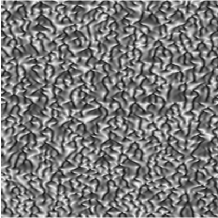
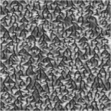
Figure 3: Space (horizontal) - time (vertical) plot of the complex amplitude modulus $|W|$ for $\mu=0.1$ (a) and $\mu=0.3$ (b). The system size is $N=400$.

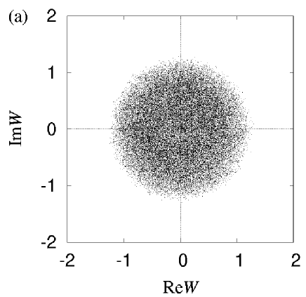
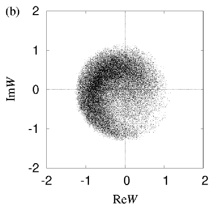
Figure 4: Phase portraits for $\mu=0.1$ (a) and $\mu=0.3$ (b) at a given time. The system size is $N=40000$.

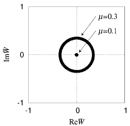
Figure 5: Trajectories of the mean field in the complex plane for $\mu=0.1$ and $\mu=0.3$. The mean field is fluctuating around the origin when $\mu=0.1$, while it forms a closed orbit with small amplitude fluctuations when $\mu=0.3$. The fluctuations come from the finiteness of the system size. The system size is $N=40000$.

The nonlinear Langevin equation (11) actually predicts the occurrence of a noisy Hopf bifurcation. From the symmetry of our system and the smallness in amplitude of the collective oscillation near its onset, the nonlinear effects ${\cal N}(\bar{W})$ in Eq. (11) will be dominated by a cubic term. Then the mean field obeys a noisy Stuart-Landau equation

$$\dot{\bar{W}}=\left[\left(\mu-\mu_{\rm c}\right)+i\omega\right]\bar{W}-\left(\eta+i\alpha\right)\left|\bar{W}\right|^{2}\bar{W}+f(t),$$ (14)

where the coefficients $\mu_{\rm c}$, $\omega$, $\eta(>0)$, and $\alpha$ are real and depend generally on $c_{1}$ and $c_{2}$. Since the above equation can be handled analytically, it would be interesting to compare some of the results from its analysis with our direct numerical simulations on Eq. (1) and its two-dimensional extension, which are the subjects of Secs. III and IV, respectively.

III Predicted critical behavior and comparison with numerical results

The nonlinear Langevin equation (14) is equivalent with the Fokker-Planck equation of the following form  ref:risken89 ; ref:kampen81 :

$$\frac{\partial}{\partial t}P\left(r,\phi,t\right) =\frac{1}{r}\frac{\partial}{\partial r}\left\{\left[-\left(\mu-\mu_{\rm c}\right)r^{2}+\eta r^{4}\right]P+\Gamma r\frac{\partial}{\partial r}P\right\}$$

$$+\left[\left(-\omega+\alpha r^{2}\right)\frac{\partial}{\partial\phi}P+\frac{\Gamma}{r^{2}}\frac{\partial^{2}}{\partial\phi^{2}}P\right].$$ (15)

Here $P(r,\phi,t)$ is the probability density for the amplitude $r$ and the phase $\phi$ of the mean field at time $t$. The above equation admits a stationary solution independent of $\phi$ given by

$$P_{\rm st}\left(r\right)=\exp\left[-\frac{\eta}{4\Gamma}\left(r^{2}-\frac{\mu-\mu_{\rm c}}{\eta}\right)^{2}\right].$$ (16)

Various moments of $r$ defined by

$$\left\langle r^{n}\right\rangle=\frac{\displaystyle\int_{0}^{\infty}r^{n}P_{\rm st}\left(r\right)rdr}{\displaystyle\int_{0}^{\infty}P_{\rm st}\left(r\right)rdr},$$ (17)

and those of the fluctuation $\delta r\equiv r-\langle r\rangle$ can be calculated ref:risken65 . In particular, in the limit of weak random force, the mean field amplitude $\langle r\rangle$ near the transition is found to depend on $\mu-\mu_{\rm c}$ as

$$\left\langle r\right\rangle=\begin{cases}A\left(\mu-\mu_{\rm c}\right)^{1/2}&\quad\left(\mu>\mu_{\rm c}\right),\\ 0&\quad\left(\mu<\mu_{\rm c}\right),\end{cases}$$ (18)

where $A$ is a constant. Similarly, the mean field fluctuation $\langle(\delta r)^{2}\rangle$ is given by

$$\left\langle(\delta r)^{2}\right\rangle\propto\left|\mu-\mu_{\rm c}\right|^{-1},$$ (19)

which holds for $\mu\gtrless\mu_{\rm c}$. It is clear that the critical exponents associated with $\langle r\rangle$ and $\langle(\delta r)^{2}\rangle$ obey the classical law or the mean field theory, reflecting the fact that the transition is caused by the applied mean field and not by the development of local order to a macroscopic scale. Still the transition is in some sense statistical in nature unlike bifurcations in deterministic dynamical systems. This is because the loss of long-range order is solely due to turbulent fluctuations, so that a full theoretical understanding of the transition phenomenon would be impossible without statistical mechanics of chemical turbulence.

Long-time averages of $r$ and $(\delta r)^{2}$ were obtained as a function of the feedback intensity from numerical simulation of Eqs. (1) and (2) with $N=200000$, and the results are shown in Figs. 6(a) and (b), respectively. By assuming that the long-time averages are identical with ensemble averages, these numerical data were fitted with the theoretical curves given by Eqs. (18) and (19), respectively, where a scale factor is used as the only adjustable parameter. Note that $\mu_{\rm c}$ is not an adjustable parameter, but is a constant given by Eq. (13).

Figure 6: $\langle r\rangle^{2}$ vs. $\mu$ (a). $N^{-1}\langle(\delta r)^{2}\rangle^{-1}$ vs. $\mu$ (b). The open circles and the solid lines are the numerical data and the theoretical curves, respectively. In each of (a) and (b), a suitable scale factor is used as an adjustable parameter to achieve a good fitting between the theory and numerical experiments. The system size is $N=200000$.

In obtaining Eq. (18) for the mean field amplitude, we considered the limit of weak random force. Let our argument be generalized to include the dependence of $\langle r\rangle$ on the noise intensity as well as on $\mu-\mu_{\rm c}$. Because the origin of the random force driving the mean field is the finiteness of the system size, the noise intensity should be inversely proportional to the system size, or

$$\Gamma=\frac{D}{N},$$ (20)

where $D$ is a constant independent of $N$. One may thus write the stationary distribution in the form

$$P_{\rm st}(r)=\exp\left[-\frac{N\eta}{4D}\left(r^{2}-\frac{\varepsilon}{\eta}\right)^{2}\right],$$ (21)

where $\varepsilon=\mu-\mu_{\rm c}$. Applying the finite-size scaling law developed in Ref. ref:pikovsky99 to the average amplitude of the mean field, we obtain a scaling form

$$\left\langle r\right\rangle=N^{-1/4}F\left(\varepsilon N^{1/2}\right),$$ (22)

where $F$ is a function (called the scaling function) depending on $\varepsilon$ and $N$ only through $\varepsilon N^{1/2}$. Equation (22) is a generalization of Eq. (18). Numerically calculated $\langle r\rangle$ for various $\varepsilon$ and $N$ confirms this scaling law. Figure 7(a) shows the dependence of the long-time average of the mean field amplitude on feedback intensity for some different values of $N$. As is seen from Fig. 7(b), all these data come to lie on an identical universal curve after the rescalings of $\langle r\rangle$ and $\varepsilon$ by $N^{1/4}$ and $N^{1/2}$, respectively. In this way, the finite-size scaling law (22) is confirmed, providing unmistakable evidence for a phase transition.

Figure 7: $\langle r\rangle$ vs. $\mu$ for some different values of $N$ (a). Rescaling of the data in (a) according to the finite-size scaling given by Eq. (22) produces a universal curve independent of $N$ (b).

IV Two-dimensional case

The one-dimensional reaction-diffusion systems which we have numerically studied in Secs. II and III are not very realistic. Especially, surface chemical reactions, such as catalytic CO oxidation on Pt, occur in two dimensions. As mentioned in the foregoing sections, the transition considered here is the mean field type, so that the nature of the transition is expected to be the same as that in one-dimensional systems. We carried out numerical simulations on the two-dimensional complex Ginzburg-Landau equation with global feedback, and obtained a clear indication of transition, although the corresponding value of $\mu_{\rm c}$ is considerably smaller than that of the one-dimensional case under the same parameter condition. Figure 8 summarizes numerical results for various $\varepsilon$ and $N$, exhibited in a similar manner to Fig. 7(b), i.e., in the form of $\langle r\rangle N^{1/4}$ vs. $\varepsilon N^{1/2}$ for different values of $N$. These data form almost an identical curve again, which we take as evidence for a transition similar to that in one-dimensional systems.

Figure 8: Similar to Fig. 7(b) but in two space dimensions. Parameter values are the same as in the one-dimensional case, i.e., $c_{1}=2.0$ and $c_{2}=-2.0$, which gives $\mu_{\rm c}\simeq 0.10$. This value is used in rescaling of the numerical data.

V Concluding remarks

Preceding the transition at which the turbulence is completely suppressed and uniform oscillations set in, a different type of transition characterized by the emergence of collective oscillations was shown to exist in the one- and two- dimensional complex Ginzburg-Landau equations with global feedback. The transition is well described phenomenologically with the noisy Stuart-Landau equation governing the mean field. Since the noise there comes from the finite-size effects, the transition becomes infinitely sharp in the limit of infinite system size. The critical exponents of this transition obey the mean field theory because the origin of cooperativity is nothing but the mean field produced by the global feedback. This also gives the reason why spatial dimension one is sufficient for giving rise to the transition. We also confirmed that the two-dimensional complex Ginzburg-Landau equation with global feedback which is more realistic also exhibits a transition of the same type.

Throughout the present paper, our analysis was confined to the case that the feedback intensity $\mu$ is real. From our ongoing study, it is being confirmed that a transition of the same nature persists over some range of complex $\mu$. The nonlinear Langevin equation (11) also seems to remain valid. Unlike the case of real $\mu$, however, the effective damping coefficient $\gamma$ appearing in the Langevin equation (11) seems to depend on $\mu$, which raises an interesting theoretical problem to be tackled in the future.

Our analysis ref:kawamura06 also suggests that the realistic dynamical model for the catalytic CO oxidation ref:kim01 ; ref:bertram03-2 under experimentally accessible parameter conditions also exhibit a similar transition. We strongly hope for its experimental verification.

- (1) D. Battogtokh and A. S. Mikhailov, Physica D 90, 84 (1996).
- (2) D. Battogtokh, A. Preusser, and A. S. Mikhailov, Physica D 106, 327 (1997).
- (3) M. Kim, M. Bertram, M. Pollmann, A. von Oertzen, A. S. Mikhailov, H. H. Rotermund, and G. Ertl, Science 292, 1357 (2001).
- (4) Y. Kuramoto, Chemical Oscillations, Waves, and Turbulence (Springer, New York, 1984; Dover, New York, 2003).
- (5) M. Bertram, C. Beta, M. Pollmann, A. S. Mikhailov, H. H. Rotermund, and G. Ertl, Phys. Rev. E 67, 036208 (2003).
- (6) M. Bertram and A. S. Mikhailov, Phys. Rev. E 67, 036207 (2003).
- (7) I. S. Aranson and L. Kramer, Rev. Mod. Phys. 74, 99 (2002).
- (8) B. I. Shraiman, A. Pumir, W. van Saarloos, P. C. Hohenberg, H. Chaté, and M. Holen, Physica D 57, 241 (1992).
- (9) D. A. Egolf and H. S. Greenside, Nature 369, 129 (1994).
- (10) H. Risken, The Fokker-Planck Equation (Springer, Berlin, 1989).
- (11) N. G. van Kampen, Stochastic Process in Physics and Chemistry (North-Holland, Amsterdam, 1981).
- (12) H. Risken, Z. Phys. 186, 85 (1965).
- (13) A. Pikovsky and S. Ruffo, Phys. Rev. E 59, 1633 (1999).
- (14) Y. Kawamura and Y. Kuramoto, Prog. Theor. Phys. Suppl. 161, 216 (2006).