Periodic Phase Synchronization in coupled chaotic oscillators

Abstract

We investigate the characteristics of temporal phase locking states observed in the route to phase synchronization. It is found that before phase synchronization there is a periodic phase synchronization state characterized by periodic appearance of temporal phase locking state and that the state leads to local negativeness in one of the vanishing Lyapunov exponents. By taking a statistical measure, we present the evidences of the phenomenon in unidirectionally and mutually coupled chaotic oscillators, respectively. And it is qualitatively discussed that the phenomenon is described by a nonuniform oscillator model in the presence of noise.

Over the past decade, synchronization in chaotic oscillators SyncOrg0 ; SyncOrg1 has received much attention because of its fundamental importance in nonlinear dynamics and potential applications to laser dynamics PSExp , electronic circuits Circuit , chemical and biological systems NeuronSync , and secure communications Secure . Synchronization in chaotic oscillators is characterized by the loss of exponential instability in the transverse direction through interaction. In coupled chaotic oscillators, it is known, various types of synchronization are possible to observe, among which are complete synchronization (CS) SyncOrg0 ; SyncOrg1 , phase synchronization (PS) PhaseSync ; Lee , lag synchronization (LS) Lag and generalized synchronization (GS) GenSync .

One of the noteworthy synchronization phenomena in this regard is PS which is defined by the phase locking between nonidentical chaotic oscillators whose amplitudes remain chaotic and uncorrelated with each other: $|\theta_{1}-\theta_{2}|\leq\mbox{const}.$ Since the first observation of PS in mutually coupled chaotic oscillators PhaseSync , there have been extensive studies in theory Lee and experiments PSExp . The most interesting recent development in this regard is the report that the interdependence between physiological systems is represented by PS and temporary phase-locking (TPL) states, e.g., (a) human heart beat and respiration HeartBeat , (b) a certain brain area and the tremor activity BrainMuscle , etc Visual ; Wavelet . Application of the concept of PS in these areas sheds light on the analysis of nonstationary bivariate data coming from biological systems which was thought to be impossible in the conventional statistical approach. And this calls new attention to the PS phenomenon.

Accordingly, it is quite important to elucidate a detailed transition route to PS in consideration of the recent observation of a TPL state in biological systems. What is known at present is that TPLLee transits to PS and then transits to LS as the coupling strength increases. On the other hand, it is noticeable that the phenomenon from nonsynchronization to PS have hardly been studied, in contrast to the wide observations of the TPL states in the biological systems.

The chief goal of this Letter is to study the characteristics of TPL states observed in the regime from nonsynchronization to PS in coupled chaotic oscillators. We report that there exists a special locking regime in which a TPL state shows maximal periodicity, which phenomenon we would call periodic phase synchronization (PPS). We show this PPS state leads to local negativeness in one of the vanishing Lyapunov exponents, taking the measure by which we can identify the maximal periodicity in a TPL state. We present a qualitative explanation of the phenomenon with a nonuniform oscillator model in the presence of noise.

We consider here the unidirectionally coupled non-identical Ros̈sler oscillators for first example:

$$\dot{x}_{1} = -\omega_{1}y_{1}-z_{1},$$

$$\dot{y}_{1} = \omega_{1}x_{1}+0.15y_{1},$$

$$\dot{z}_{1} = 0.2+z_{1}(x_{1}-10.0),$$

$$\dot{x}_{2} = -\omega_{2}y_{2}-z_{2},$$

$$\dot{y}_{2} = \omega_{2}x_{2}+0.165y_{2}+\epsilon(y_{1}-y_{2}),$$

$$\dot{z}_{2} = 0.2+z_{2}(x_{2}-10.0),$$ (1)

where the subscripts imply the oscillators 1 and 2, respectively, $\omega_{1,2}$ $(=1.0\pm 0.015)$ is the overall frequency of each oscillator, and $\epsilon$ is the coupling strength. It is known that PS appears in the regime $\epsilon\geq\epsilon_{c}$ and that $2\pi$ phase jumps arise when $\epsilon<\epsilon_{c}$. Lyapunov exponents play an essential role in the investigation of the transition phenomenon with coupled chaotic oscillators and as generally understood that PS transition is closely related to the transition to the negative value in one of the vanishing Lyapunov exponents SyncOrg1 .

Figure 1 shows two largest conditional Lyapunov exponents from Eq. (1) according to the coupling strength $\epsilon$. One can see the dip characterized by the local negativeness in the vanishing Lyapunov exponent. The reference points A and C indicate the borders of the dip and B its center. PS transition occurs in the right of C ($\epsilon=0.085$) where the phase difference of coupled chaotic oscillators is bounded within a constant. The temporal behaviors at the three reference points are presented in Fig. 2. The phase jumps at B looks quite regular, compared to those of A and C. Though this observation may seem rather intuitive, we shall see that it is a valid one and that all the phenomenon is deeply related to the dip, the local negativeness in the vanishing Lyapunov exponent of Fig. 1.

Figure 1: Two largest conditional Lyapunov exponents and the dip in coupled Rössler oscillators when $\omega_{0}=1.0$: A ($\epsilon=0.058$), B($\epsilon=0.072$), and C ($\epsilon=0.083$) are the reference points to explain different characteristics of phase dynamics.

A vanishing Lyapunov exponent corresponds to a phase variable of an oscillator and it exhibits the neutrality of an oscillator in the phase direction. Accordingly, the local negativeness of an exponent indicates this neutrality is locally broken PhaseSync . It is important to define an appropriate phase variable in order to study the TPL state more thoroughly. In this regard, several methods have been proposed methods of using linear interpolation at a Poincaré section PhaseSync , phase space projection PhaseSync ; Lee , tracing of the center of rotation in phase space Spline , Hilbert transformation PhaseSync ; Wavelet , or wavelet transformation Wavelet . Among these we take the method of phase space projection onto the $x_{1}-y_{1}$ and $x_{2}-y_{2}$ planes with the geometrical relation $\theta_{1,2}=\arctan(y_{1,2}/x_{1,2})$, and obtain phase difference $\phi=\theta_{1}-\theta_{2}$.

The system of coupled oscillators is said to be in a TPL state (or laminar state) when $\langle\dot{\phi}\rangle<\Lambda_{c}$ where $\langle...\rangle$ is the running average over appropriate short time scale and $\Lambda_{c}$ is the cutoff value to define a TPL state. The locking length of the TPL state, $\tau$, is defined by time interval between two adjacent peaks of $\langle\dot{\phi}\rangle$ (see Fig. 2).

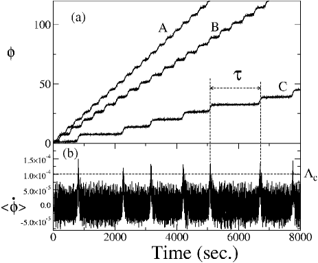
Figure 2: Temporal behaviors of the phase difference: (a) $\phi$ at each reference point. $\tau$ is the locking length of a TPL state. (b) $\langle\dot{\phi}\rangle$ at reference point C (running averaged over 10 seconds to remove irrelevant fast fluctuations). The cutoff value for TPL a state is $\Lambda_{c}=1.0\times 10^{-4}$.

In order to study the characteristics of the locking length $\tau$, we introduce a measure:

$$P(\epsilon)=\frac{\sqrt{\mbox{var}(\tau)}}{\langle\tau\rangle},$$ (2)

which is the ratio between the average value of time lengths of TPL states and their standard deviation. In terminology of stochastic resonance, it can be interpreted as noise-to-signal ratio Coherence ; SR . The measure would be minimized where the periodicity is maximized in TPL states.

Figure 3: Measure P as a function of $\epsilon$. Big dots are the reference points of Fig.1 and each point is the average value of 2500 TPL states.

Measure $P$ as a function of $\epsilon$ is presented in Fig. 3. The big dots indicate the reference points of Fig. 1. We see that the value of P begins to drop rapidly from reference point A which corresponds to the left border of the dip in Fig. 1. And the value of $P$ is minimized in a broad region around B, the center of the dip. The value rapidly increases after passing reference point C, the right border of the dip. What is interesting here is that in the region from $\epsilon=0.062$ to $0.078$ the periodicity is maximized and corresponds to the central part of the dip. Eventually, the coupled chaotic oscillators develop to PS near $\epsilon=0.085$. The result presented in Fig. 3 leads us to argue that the dip in a vanishing Lyapunov exponent shows the maximal periodicity of TPL states around the minimum of $P$. We call the TPL state inside the dip a PPS state in the sense that the TPL state appears rather periodically than outside the dip.

To validate the argument, we explain the phenomenon in simplified dynamics. From Eq. (1), we obtain the equation of motion in terms of phase difference:

$$\frac{d\phi}{dt} = \Delta\omega+A(\theta_{1},\theta_{2},\epsilon)\sin\phi+\xi(\theta_{1},\theta_{2},\epsilon),$$ (3)

where,

$$A(\theta_{1},\theta_{2},\epsilon) = (\epsilon+0.15)\cos(\theta_{1}+\theta_{2})-\frac{\epsilon}{2}(\frac{R_{1}}{R_{2}}),$$

$$\xi(\theta_{1},\theta_{2},\epsilon) = \frac{\epsilon}{2}\frac{R_{1}}{R_{2}}\sin(\theta_{1}+\theta_{2})+\frac{z_{1}}{R_{1}}\sin(\theta_{1})-\frac{z_{2}}{R_{2}}\sin(\theta_{2})$$

$$+(\epsilon+0.015)\cos(\theta_{2})\sin(\theta_{2}).$$

Here $\Delta\omega=\omega_{1}-\omega_{2}$ and $R_{1,2}=\sqrt{x_{1,2}^{2}+y_{1,2}^{2}}$. And from Eq. (3) we obtain the simplified equation to describe the phase dynamics: ${d\phi}/{dt}=\Delta\omega+\langle A\rangle\sin(\phi)+\xi$, where $\langle A\rangle$ is the time average of $A(\theta_{1},\theta_{2},\epsilon)$. This is a nonuniform oscillator in the presence of noise where $\xi$ plays a role of effective noise Strogatz and the value of $\langle A\rangle$ controls the width of bottleneck (i.e, nonuniformity of the flow). If the bottleneck is wide enough, (i.e., faraway from the saddle-node bifurcation point: $\Delta\omega\gg-\langle A\rangle$), the effective noise hardly contributes to the phase dynamics of the system. So the passage time is wholly governed by the width of the bottleneck as follows: $\langle\tau\rangle\sim 1/\sqrt{\Delta\omega^{2}-\langle A\rangle^{2}}\sim 1/\sqrt{\Delta\omega^{2}-\epsilon^{2}/4}$, which is a slowly increasing function of $\epsilon$. In this region while the standard deviation of TPL states is nearly constant (because the widely opened bottlenecks periodically appears and those lead to small standard deviation), the average value of locking length of TPL states is relatively short and the ratio between them is still large. Accordingly, the value of $P(\epsilon)$ slowly decreases in the regime before reference point B in Fig. 3.

On the contrary as the bottleneck becomes narrower (i.e., near the saddle-node bifurcation point: $\Delta\omega\geq-\langle A\rangle$) the effective noise begins to perturb the process of bottleneck passage and regular TPL states develop into intermittent ones (see C in Fig. 2 (a)) Lee ; Kye . It makes the standard deviation increase very rapidly and this trend overpowers that of the average value of locking lengths of the TPL states. For that reason, the value of $P(\epsilon)$ rapidly increases passing the PPS regime in Fig. 3. Thus we understand that the competition between width of bottleneck and amplitude of effective noise produces the crossover at the minimum point of $P(\epsilon)$ which shows the maximal periodicity of TPL states.

Figure 4: Lyapunov exponents and measure P in mutually coupled Rössler oscillator: $\dot{x}_{1,2}=-\omega_{1,2}y_{1,2}-z_{1,2}+\epsilon(x_{2,1}-x_{1,2}),\dot{y}_{1,2}=\omega_{1,2}x_{1,2}+0.15y_{1,2},\dot{z}_{1,2}=0.2+z_{1,2}(x_{1,2}-10.0)$, where $\omega_{1,2}=1.0\pm 0.015$. (a) One can see the dip in one of the vanishing Lyapunov exponents and the reference point D indicates the center of it. (b) The big dot shows the minimum point and it coincides with the point of the center of the dip. Each point is the average value of 12000 TPL states.

Rosenblum et al. firstly observed the dip in mutually coupled chaotic oscillators PhaseSync . However the origin and the dynamical characteristics of the dip have been left unclarified. We argue that the dip observed in mutually coupled chaotic oscillators has the same origin as observed above in unidirectionally coupled systems. Figure 4 shows the four largest Lyapunov exponents and the value of $P$ according to the coupling strength $\epsilon$. We can see that the minimum region of $P$ from $\epsilon=0.022$ to $0.027$ coincides with the central part of the dip (D in the figure) even though the valley in Fig. 4 (b) is not deeper than that of the unidirectionally coupled systems. Thus it is reasonably summed up that a PPS state exists just before the transition to PS and that the dip observed by Rosenblum et al. is the very evidence of a PPS state in mutually coupled chaotic oscillators.

Common apprehension is that near the border of synchronization the phase difference in coupled regular oscillators is periodic PhaseSync whereas in coupled chaotic oscillators it is irregular Lee . On the contrary, we report that the special locking regime exhibiting the maximal periodicity of a TPL state also exists in the case of coupled chaotic oscillators. In general, the phase difference of coupled chaotic oscillators is described by the one-dimensional Langevin equation: $\dot{\phi}=F(\phi)+\xi$ where $\xi$ is the effective noise with finite amplitude. The investigation with regard to PS transition is the study of scaling of the laminar length around the virtual fixed point $\phi^{*}$ where $F(\phi^{*})=0$ Kye ; Virtual and PS transition is established when $|\int^{\phi^{*}}_{\phi}F(\phi)d\phi|>\max|\xi|$. Consequently, the crossover region, from which the value of $P$ grows exponentially (as shown in Fig. 3-4), exists because intermittent series of TPL states with longer locking length $\tau$ appears as PS transition is nearer. Eventually it leads to an exponential growth of the standard deviation of the locking length. Thus we argue that PPS is the generic phenomenon mostly observed in coupled chaotic oscillators prior to PS transition.

In conclusion, analyzing the dynamic behaviors in coupled chaotic oscillators with slight parameter mismatch we have completed the whole transition route to PS. We find that there exists a special locking regime called PPS in which a TPL state shows maximal periodicity and that the periodicity leads to local negativeness in one of the vanishing Lyapunov exponents. We have also made a qualitative description of this phenomenon with the nonuniform oscillator model in the presence of noise. Investigating the characteristics of TPL states between nonsynchronization and PS, we have clarified the transition route before PS. Since PPS appears in the intermediate regime between non-synchronization and PS, we expect that the concept of PPS can be used as a tool for analyzing weak interdependences, i.e. those not strong enough to develop to PS, between nonstationary bivariate data coming from biological systems, for instance. Moreover PPS could be a possible mechanism of the chaos regularization phenomenon Regular ; Regular1 observed in neurobiological experiments.

Note added. - Recently, we were informed by S. Boccaletti that the phenomenon observed by us was confirmed in CO₂ laser systems, experimentally Bocca .

The authors acknowledge the correspondence with S. Boccaletti, E. Allaria, R. Meucci, and F.T. Arecchi about experimental confirmation of PPS and thank A. Pikovsky, Y. -C. Lai, K. Josić, and M. Choi for helpful comments. This work is supported by Creative Research Initiatives of the Korean Ministry of Science and Technology.

References

- (1) H. Fujisaka and T. Yamada, Prog. Theor. Phys. 69, 32 (1983); V. S. Afraimovich, N. N. Verichev, and M. I, Rabinovich, Radiophys. Quantum Electron. 29, 747 (1986).
- (2) L. M. Pecora and T. L. Carroll, Phys. Rev. Lett. 64, 821 (1990)
- (3) D. J. DeShazer, R. Breban, E. Ott, and R. Roy, Phys. Rev. Lett. 87, 044101(2001); K. V. Volodchenko, V. N. Ivanov, and S.-H. Gong et al., Optics Letters 26, 1406 (2001).
- (4) C. M. Kim, G. S. Yim, J. W. Ryu, and Y. J. Park, Phys. Rev. Lett. 80; L. Zhu and Y.-C. Lai, Phys. Rev. E 64, 045205 (2001).
- (5) R. C. Elson, A. I. Selverston, and R. Huerta et al., Phys. Rev. Lett. 81, 5692 (1998).
- (6) L. Kocarev and U. Parlitz, Phys. Rev. Lett. 74, 5028 (1995) and references therein.
- (7) M. Rosenblum, A. Pikovsky, and J. Kurths, Phys. Rev. Lett. 76, 1804 (1996); A. Pikovsky, M. Rosenblum, and J. Kurths, Synchronization A universal concept in nonlinear sciences, Cambridge University Press 2001.
- (8) K.J. Lee, Y. Kwak, and T.K. Lim, Phys. Rev. Lett. 81, 321 (1998); E. Rosa, E. Ott, and M.H. Hess, Phys. Rev. Lett. 80, 1642 (1998); K. Josić and D.J. Mar, Phys. Rev. E64, 056234 (2001).
- (9) M. Rosenblum, A. Pikovsky and J. Kurths, Phys. Rev. Lett. 78, 4193 (1997).
- (10) L. Kocarev and U. Parlitz, Phys. Rev. Lett. 76, 1816 (1996).
- (11) C. Schäfer, M.G. Rosenblum, J. Kurths, and H.-H Abel, Nature 392 239 (1998); C. Schäfer, M.G. Rosenblum, H.-H Abel, and J. Kurths, Phys. Rev. E 60, 857 (1999).
- (12) P. Tass, M. G. Rosenblum, J, Weule, J. Kurths et al., Phys. Rev. Lett. 81, 3291 (1998).
- (13) E. Rodriguez, N. George, J. Lachaux, J. Martinerie, B. Renault and F. Varela, Nature, 397, 430 (1999).
- (14) R. Q. Quiroga, A. Kraskov, T. Kreuz, and P. Grassberger, arXiv:nln.CD/0109023.
- (15) T. Yalcinkaya and Y. -C. Lai, Phys. Rev. Lett. 79, 3885 (1997).
- (16) S. H. Strogatz, NONLINEAR DYNAMICS AND CHAOS, PERSEUS BOOKS, 1998.
- (17) A. Pikovsky and J. Kurth, Phys. Rev. Lett. 78, 775 (1997).
- (18) P. Jung, Phys. Reports 234, 175 (1993).
- (19) W.-H. Kye and C.-M. Kim, Phys. Rev. E 62, 6304 (2000).
- (20) W.-H. Kye and D. Topaj, Phys. Rev. E 63, 045202(R) (2001).
- (21) The Stomatogastric Nervous System, edited by R.M. Harris-Warrick et al. (MIT Press, Cambridge, MA, 1992); M.I. Rabinovich et al., IEEE Trans. Circuits Syst.-I 44, 997 (1997).
- (22) N. F. Rulkov, Phys. Rev. Lett. 86, 183 (2001) and references therein.
- (23) S. Boccaletti, E. Allaria, R. Meucci and F. T. Arrecchi, Phys. Rev. Lett. 89, 194101 (2002); private communication.