Probabilistic cellular automata with conserved quantities

1 Introduction

Cellular automata (CA) are dynamical systems characterized by discreteness in space and time. In general, they can be viewed as cells in a regular lattice updated synchronously according to a local interaction rule, where the state of each cell is restricted to a finite set of allowed values.

As in any other dynamical system, conservation laws play an important role in CA. Additive invariants in one-dimensional CA have been studied by Hattori and Takesue [1]. They obtained conditions which guarantee the existence of additive conserved quantities, and produced a table of additive invariants for Wolfram’s elementary CA rules. The simplest of additive invariants, namely the number of active sites (“active” meaning non-zero), plays especially important role in CA dynamics. CA possessing such invariant, to be called “conservative CA”, can be viewed as a system of interacting particles, as described in [2]. In a finite system, the flux or current of particles in equilibrium depends only on their density, which is invariant. The graph of the current as a function of density characterizes many features of the flow, and is therefore called the fundamental diagram. Fundamental diagrams of conservative CA were investigated in [3, 4]. For majority of conservative CA rules, fundamental diagrams are piecewise-linear, usually possessing one or more “sharp corners” or singularities. Although the shapes of fundamental diagrams vary, there is a strong evidence of the universal behavior at singularities, as reported in [5].

Conservative CA appear in various applications, and some special cases have been studied extensively. Rule 184, which is a discrete version of the totally asymmetric exclusion process, is a prime example of such special case [6, 7, 8, 9, 10, 11, 12, 13, 14]. Although much is known about this particular rule, dynamics of other conservative rules exhibits many features which are not fully understood, and more general results are just starting to appear. For example, M. Pivato [15] recently studied conservation laws in CA in a very general setting, deriving both theoretical consequences and practical tests for conservation laws, and provided a method for constructing all one-dimensional CA exhibiting a given conservation law. Another recent work [16] investigates universality and decidability of conservative CA. Unfortunately, there exists no general result explaining the shape of fundamental diagrams for conservative CA’s, in spite of a remarkable progress reported recently for a special class of rules [17].

In this paper, we will introduce a natural extension of the conservation condition to include probabilistic cellular automata (PCA). Deterministic conservative rules will then become a special case of conservative PCA. For the nearest-neighbour case, this allows to parameterize all conservative PCA by a set of three parameters. In the three-dimensional parameter space, nearest-neighbour conservative PCA are represented by a polyhedron, with deterministic rules located at its vertices. We will then show that the general shape of the fundamental diagram for nearest-neighbour PCA can be partially explained by a mean-field type approximation.

2 Probabilistic boolean CA

In what follows, we will assume that the dynamics takes place on a one-dimensional lattice of length $L$ with periodic boundary conditions. Let $s_{i}(k)$ denote the state of the lattice site $i$ at time $k$, where $i\in\{0,1,\ldots,L-1\}$, $k\in{\mathbf{N}}$. All operations on spatial indices $i$ are assumed to be modulo $L$. We will further assume that $s_{i}(k)\in\{0,1\}$, and we will say that the site $i$ is occupied (empty) at time $k$ if $s_{i}(k)=1$ ($s_{i}(k)=0$). We will also define $\mathbf{s}(k)=\{s_{0}(k),s_{1}(k),\ldots,s_{L-1}(k)\}$.

In a probabilistic cellular automaton, lattice sites simultaneously change states form $0$ to $1$ or from $1$ to $0$ with probabilities depending on states of local neighbours. A common method for defining PCA is to specify a set of local transition probabilities. For example, in order to define a nearest-neighbour PCA one has to specify the probability $w(s_{i}(k+1))|s_{i-1}(k),s_{i}(k),s_{i+1}(k))$ that the site $s_{i}(k)$ with nearest neighbors $s_{i-1}(k),s_{i+1}(k)$ changes its state to $s_{i}(k+1)$ in a single time step. For the sake of illustration, consider a recently investigated PCA rule [18], where empty sites become occupied with a probability proportional to the number of occupied sites in the neighborhood, and occupied sites become empty with a probability proportional to the number of empty sites in the neighborhood. The following set of transition probabilities defines the aforementioned PCA rule:

$$w(1|0,0,0) =0 \qquad w(1|0,0,1) =p$$

$$w(1|0,1,0) =1-2p \qquad w(1|0,1,1) =1-p$$

$$w(1|1,0,0) =p \qquad w(1|1,0,1) =2p$$

$$w(1|1,1,0) =1-p \qquad w(1|1,1,1) =1,$$ (1)

where $p\in[0,1/2]$. The remaining eight transition probabilities can be obtained using $w(0|a,b,c)=1-w(1|a,b,c)$ for $a,b,c\in\{0,1\}$.

We will now proceed to construct a general definition of PCA, with arbitrary neighbourhood size. Let $n$ be a positive integer, and let $C=\{c_{1},c_{2},\ldots,c_{n}\}$ be a set of integers such that $c_{i+1}=c_{i}+1$ for all $i=1\ldots n-1$. The set $\{s_{i+c_{1}}(k),s_{i+c_{2}}(k),\ldots,s_{i+c_{n}}(k)\}$ will be called a neighbourhood of the site $s_{i}(k)$. We will assume that the neighbourhood always includes the site $s_{i}(k)$, i.e., $c_{1}\leq 0$.

Consider now a set of independent Boolean random variables $X_{i,\mathbf{v}}$, where $i=0,1,\ldots L-1$ and $\mathbf{v}\in\{0,1\}^{n}$. Probability that the random variable $X_{i,\mathbf{v}}$ takes the value $a\in\{0,1\}$ will be denoted by $w(a|\mathbf{v})$,

$$Pr(X_{i,\mathbf{v}}=a)=w(a|\mathbf{v}).$$ (2)

Obviously, $w(1|\mathbf{v})+w(0|\mathbf{v})=1$ for all $\mathbf{v}\in\{0,1\}^{n}$. The update rule for PCA is defined by

$$s_{i}(k+1)=X_{i,\{s_{i+c_{1}}(k),s_{i+c_{2}}(k),\ldots,s_{i+c_{n}}(k)\}}.$$ (3)

Note that $\{\mathbf{s}(k):k=0,1,2,\ldots\}$ is a Markov stochastic process, and its states are binary sequences $\mathbf{s}(k)\in\{0,1\}^{L}$. The probability of transition from $\mathbf{x}\in\{0,1\}^{L}$ to $\mathbf{y}\in\{0,1\}^{L}$ in one time step is given by

$$Pr(\mathbf{y}|\mathbf{x})=\prod_{i=0}^{L-1}w(y_{i}|\{x_{i+c_{1}},x_{i+c_{2}},\ldots,x_{i+c_{n}}\}).$$ (4)

To illustrate the above formalism, let us consider again the rule (2) defined at the beginning of this section. For this rule, we have $C=\{-1,0,1\}$, and each lattice site $i$ is associated with eight random variables $X_{i,000}$, $X_{i,001}$, $X_{i,010}$, $X_{i,011}$, $X_{i,100}$, $X_{i,101}$, $X_{i,110}$, and $X_{i,111}$. Probability distributions of these r.v. are determined by (2). For instance, $w(1|1,0,0)=p$, and therefore we have $Pr\big{(}X_{i,100}=1\big{)}=p$, and $Pr\big{(}X_{i,100}=0\big{)}=1-p$. Similarly, $w(1|0,0,0)=0$, hence $Pr\big{(}X_{i,000}=1\big{)}=0$ and $Pr\big{(}X_{i,000}=0\big{)}=1$, meaning that $X_{i,000}$ is in this case a deterministic variable.

3 Conservative rules

If for any initial distribution $\mu$

$$E_{\mu}\left(\sum_{i=0}^{L-1}s_{i}(k)\right)=E_{\mu}\left(\sum_{i=0}^{L-1}s_{i}(k+1)\right)$$ (5)

for all $k=0,1,\ldots$, then the PCA defined by (3) will be called conservative. The expectation value of the sum $\sum_{i=0}^{L-1}s_{i}(k)$ can be interpreted as the expected number of sites occupied by “particles”, therefore the condition (5) requires that the expected number of “particles” in the system is constant.

Since the expected value of the random variable $X_{i,\mathbf{v}}$ depends only on the vector $\mathbf{v}$, we will now define function $f:\{0,1\}^{n}\rightarrow[0,1]$ as

$$f(x_{1},x_{2},\ldots,x_{n})=E\left(X_{i,\{x_{1},x_{2},\ldots,x_{n}\}}\right).$$ (6)

Proposition 1

The probabilistic CA rule defined by (3) is conservative if and only if

$$\sum_{i=0}^{L-1}f(x_{i},x_{i+1},\ldots,x_{i+n-1})=\sum_{i=0}^{L-1}x_{i}$$ (7)

for all $\{x_{0},x_{1},\ldots,x_{L-1}\}\in\{0,1\}^{L}$.

Proof. To prove that (5) implies (7), it is enough to choose deterministic initial configuration, $s_{0}(0)=x_{0}$, $s_{1}(0)=x_{1}$, …, $s_{L-1}(0)=x_{L-1}$ for any $\{x_{0},x_{1},\ldots,x_{L-1}\}\in\{0,1\}^{L}$. Then

$$E_{\mu}\left(\sum_{i=0}^{L-1}s_{i}(0)\right)=\sum_{i=0}^{L-1}x_{i},$$ (8)

and using (3)

$$E_{\mu}\left(\sum_{i=0}^{L-1}s_{i}(1)\right)=\sum_{i=0}^{L-1}E_{\mu}\left(X_{i,\{s_{i+c_{1}}(0),s_{i+c_{2}}(0),\ldots,s_{i+c_{n}}(0)\}}\right)\\ =\sum_{i=0}^{L-1}E_{\mu}\left(X_{i,\{x_{i+c_{1}},x_{i+c_{2}},\ldots,x_{i+c_{n}}\}}\right)=\sum_{i=0}^{L-1}f(x_{i+c_{1}},x_{i+c_{2}},\ldots,x_{i+c_{n}}\})\\ =\sum_{j=0}^{L-1}f(x_{j},x_{j+1},\ldots,x_{j+n-1}),$$ (9)

where $j=i+c_{1}$. Condition (5) requires that $E_{\mu}\left(\sum_{i=0}^{L-1}s_{i}(0)\right)$ and $E_{\mu}\left(\sum_{i=0}^{L-1}s_{i}(1)\right)$ must be equal, hence (7) follows.

In order to prove that (7) implies (5), we will use the definition of the expectation value

$$E_{\mu}\left(\sum_{i=0}^{L-1}s_{i}(k+1)\right)=\sum_{\mathbf{x}\in\{0,1\}^{L}}Pr\big{(}\mathbf{s}(k+1)=\mathbf{x}\big{)}\sum_{i=0}^{L-1}x_{i},$$ (10)

where $\mathbf{x}=\{x_{0},x_{1},\ldots,x_{L-1}\}$. Probability $Pr\big{(}\mathbf{s}(k+1)=\mathbf{x}\big{)}$ can be written as

$$Pr\big{(}\mathbf{s}(k+1)=\mathbf{x}\big{)}=\sum_{\mathbf{y}\in\{0,1\}^{L}}Pr(\mathbf{x}|\mathbf{y})Pr\big{(}\mathbf{s}(k)=\mathbf{y}\big{)}$$ (11)

where $Pr(\mathbf{x}|\mathbf{y})$ denotes the probability of transition from $\mathbf{y}$ to $\mathbf{x}$ in a single time step. Combining the above two equations and changing the order of summation we obtain

$$E_{\mu}\left(\sum_{i=0}^{L-1}s_{i}(k+1)\right)\\ =\sum_{\mathbf{x}\in\{0,1\}^{L}}\sum_{\mathbf{y}\in\{0,1\}^{L}}Pr\big{(}\mathbf{s}(k)=\mathbf{y}\big{)}Pr(\mathbf{x}|\mathbf{y})\sum_{i=0}^{L-1}x_{i}\\ =\sum_{\mathbf{y}\in\{0,1\}^{L}}Pr\big{(}\mathbf{s}(k)=\mathbf{y}\big{)}\sum_{i=0}^{L-1}\sum_{\mathbf{x}\in\{0,1\}^{L}}Pr(\mathbf{x}|\mathbf{y})\,x_{i}.$$ (12)

Note that the last sum, $\sum_{\mathbf{x}\in\{0,1\}^{L}}Pr(\mathbf{x}|\mathbf{y})\,x_{i}$, is simply equal to the expected value of $x_{i}$ given the previous state of the system $\mathbf{y}$. This expected value must be equal to

$$E\left(X_{i,\{y_{i+c_{1}},y_{i+c_{2}},\ldots,y_{i+c_{n}}\}}\right)=f(y_{i+c_{1}},y_{i+c_{2}},\ldots,y_{i+c_{n}}),$$ (13)

and as a consequence we have

$$E_{\mu}\left(\sum_{i=0}^{L-1}s_{i}(k+1)\right)\\ =\sum_{\mathbf{y}\in\{0,1\}^{L}}Pr\big{(}\mathbf{s}(k)=\mathbf{y}\big{)}\sum_{i=0}^{L-1}f(y_{i+c_{1}},y_{i+c_{2}},\ldots,y_{i+c_{n}})\\ =\sum_{\mathbf{y}\in\{0,1\}^{L}}Pr\big{(}\mathbf{s}(k)=\mathbf{y}\big{)}\sum_{i=0}^{L-1}y_{i}\\ =E_{\mu}\left(\sum_{i=0}^{L-1}s_{i}(k)\right),$$ (14)

precisely what we wanted to show. $\square$

Following [1, 4], it is possible to obtain a simple condition which a probabilistic conservative CA rule must satisfy.

Proposition 2

A probabilistic CA rule $f$ is number-conserving if, and only if, for all $\{x_{1},x_{2},\ldots,x_{n}\}\in\{0,1\}^{n}$, it satisfies

$$f(x_{1},x_{2},\ldots,x_{n})=x_{1}+\sum_{k=1}^{n-1}\big{(} f(\underbrace{0,0,\ldots,0}_{k},x_{2},x_{3},\ldots,x_{n-k+1})$$

$$- f(\underbrace{0,0,\ldots,0}_{k},x_{1},x_{2},\ldots,x_{n-k})\big{)}.$$ (15)

Proof. To prove that Condition (15) is necessary, we will first note that $f(0,0,\ldots,0)=0$, which is a direct consequence of the condition (7) applied to the configuration consisting of all zeros, $\{x_{0},x_{1},\ldots,x_{L-1}\}=\{0,0,\ldots,0\}$. Consider now a configuration of length $L\geq 2n-1$ which is the concatenation of a sequence $\{x_{1},x_{2},\ldots,x_{n}\}$ and a sequence of $L-n$ zeros. If $f$ is conservative, such configuration must satisfy condition (7), hence

$$f(0,0,\ldots,0,x_{1}) +f(0,0,\ldots,0,x_{1},x_{2})+\cdots$$

$$\qquad+f(x_{1},x_{2},\ldots,x_{n})+f(x_{2},x_{3},\ldots,x_{n},0)+\cdots$$

$$\qquad+f(x_{n},0,\ldots,0)=x_{1}+x_{2}+\cdots+x_{n},$$ (16)

where all the terms of the form $f(0,0,\ldots,0)$, which are equal to zero, have not been written.

Replacing $x_{1}$ by 0 in (16) gives

$$f(0,0,\ldots,0,x_{2}) +\cdots+f(0,x_{2},\ldots,x_{n})$$

$$+f(x_{2},x_{3},\ldots,x_{n},0)+\cdots+f(x_{n},0,\ldots,0)$$

$$=x_{2}+\cdots+x_{n}.$$ (17)

Subtracting (17) from (16) yields (15).

To prove that condition (15) is sufficient, we can apply it to each site $x_{i}$ of a configuration $\{x_{0},x_{1},\ldots,x_{L-1}\}$,

$$f(x_{i+1},x_{i+2},\ldots,x_{i+n})\\ =x_{i+1}+\sum_{k=1}^{n-1}\big{(}f(\underbrace{0,0,\ldots,0}_{k},x_{i+2},x_{i+3},\ldots,x_{i+n-k+1})\\ -f(\underbrace{0,0,\ldots,0}_{k},x_{i+1},x_{i+2},\ldots,x_{i+n-k})\big{)}.$$ (18)

Obviously, when the above is summed over $i\in\{0,1,\ldots,L-1\}$, all the right-hand side terms except the first cancel, and we obtain (7). $\square$

Local mappings $f$ for conservative PCA exhibit some interesting symmetries. We have already demonstrated that $f(0,0,\ldots,0)=0$, and one can easily show that similar property is true when we replace zeros by ones, i.e., $f(1,1,\ldots,1)=1$. The following proposition shows yet another symmetry.

Proposition 3

If a mapping $f:\{0,1\}^{n}\rightarrow[0,1]$ represents conservative PCA rule, then

$$\sum_{x_{1},x_{2},\ldots,x_{n}\in\{0,1\}}f(x_{1},x_{2},\ldots,x_{n})=2^{n-1}.$$ (19)

We will say that $f$ satisfying the above condition is $1$-balanced.

Proof. Consider a configuration $\mathbf{t}=\{t_{0},t_{1},\ldots,t_{L-1}\}\in\{0,1\}^{L}$, where $L=2^{n}$. Now, let us construct a set of sequences of length $n$, $A=\{\mathbf{b}^{(j)}\}_{j=0}^{L-1}$ such that $\mathbf{b}^{(j)}=\{t_{j},t_{j+1},\ldots,t_{j+n-1}\}$. Superscript $(j)$ denotes here just a consecutive number of the sequence $\mathbf{b}^{(j)}$ in the set $A$. Recall that all operations on subscript indices are taken modulo $L$.

Assume that we can find $\mathbf{t}$ such that all sequences in $A$ are different. This means that each possible sequence of length $n$ occurs in $A$ once and only once, and therefore

$$\sum_{x_{1},x_{2},\ldots,x_{n}\in\{0,1\}}f(x_{1},x_{2},\ldots,x_{n})=\sum_{i=0}^{L-1}f(t_{i},t_{i+1},\ldots,t_{i+n-1})=N_{1},$$ (20)

where $N_{1}$ is the number of 1’s in the sequence $\mathbf{t}$.

On the other hand, $\bar{\mathbf{t}}\in\{0,1\}^{L}$, which is obtained from $\mathbf{t}$ by replacing all zeros by ones and vice versa, must also have the same property as $\mathbf{t}$, i.e.,

$$\sum_{x_{1},x_{2},\ldots,x_{n}\in\{0,1\}}f(x_{1},x_{2},\ldots,x_{n})=\sum_{i=0}^{L-1}f(\bar{t}_{i},\bar{t}_{i+1},\ldots,\bar{t}_{i+n-1})=N_{0},$$ (21)

where $N_{0}$ is the number of 0’s in $\mathbf{t}$. Comparing (20) and (21) we obtain $N_{0}=N_{1}=2^{n}/2=2^{n-1}$, exactly as required.

The only problem left is to show that, indeed, for any $n>0$, we can construct the sequence $\mathbf{t}$ of length $2^{n}$ (with periodic boundary conditions) such that all subsequences of length $n$ occurring in $t$ are different (and therefore, constitute a set of all possible sequences of length $n$). For example, for $n=3$, $\mathbf{t}=11101000$ is the required sequence. One can see that sequences of length $3$ occurring in $\mathbf{t}$, $111$, $110$, $101$, $010$, $100$, $000$, $001$, and $011$, are all possible binary sequences of length $3$.

For a general $n$, the required $\mathbf{t}$ is equivalent to a hamiltonian cycle in the de Bruijn graph [19] of dimension $n$ (or an eulerian cycle in the de Bruijn graph of dimension $n-1$). It can be demonstrated that such a cycle always exists (more precisely, for a given $n$, there exist exactly $2^{2^{n-1}-n}$ of such cycles – see, for example, review article [20]). $\square$

4 Example: nearest neighbour conservative PCA

We will now consider the case of nearest-neighbour PCA, for which the neighbourhood is defined by $C=\{-1,0,1\}$. The most general PCA of this type is defined by eight parameters $w(1|abc)\in[0,1]$ for $a,b,c\in\{0,1\}$:

$$f(0,0,0) =w(1|000), \qquad f(1,0,0) =w(1|100),$$

$$f(0,0,1) =w(1|001), \qquad f(1,0,1) =w(1|101),$$

$$f(0,1,0) =w(1|010), \qquad f(1,1,0) =w(1|110),$$

$$f(0,1,1) =w(1|011), \qquad f(1,1,1) =w(1|111).$$ (22)

Remaining eight probabilities can be determined by using consistency condition $w(0|abc)+w(1|abc)=1$. Proposition 2 imposes extra conditions on $f$,

$$f(x_{1},x_{2},x_{3})=x_{1}+f(0,x_{2},x_{3})+f(0,0,x_{2})-f(0,x_{1},x_{2})-f(0,0,x_{1}),$$ (23)

for all $x_{1},x_{2},x_{3}\in\{0,1\}$. Writing these conditions explicitly, one obtains eight equations, among them only five are independent, implying that there are three free parameters in the solution. The general solution parameterized by $\alpha$, $\beta$ and $\gamma$ is given by

$$f(0,0,0) =w(1|000)=0, \quad f(1,0,0) =w(1|100)=\alpha,$$

$$f(0,0,1) =w(1|001)=\beta, \quad f(1,0,1) =w(1|101)=\alpha+\beta,$$

$$f(0,1,0) =w(1|010)=1-\alpha-\beta, \quad f(1,1,0) =w(1|110)=1-\beta+\gamma,$$

$$f(0,1,1) =w(1|011)=1-\alpha-\gamma, \quad f(1,1,1) =w(1|111)=1,$$ (24)

where the three free parameters $\alpha,\beta,\gamma$ satisfy conditions

$$\alpha\geq 0,\quad\beta\geq 0,\quad\alpha+\beta\leq 1,\quad\alpha+\gamma\leq 1,\quad\beta-\gamma\leq 1,$$ (25)

so that all probabilities $w(1|abc)$ remain in the interval $[0,1]$. One can easily show that the following single expression for $f(x_{1},x_{2},x_{3})$ is equivalent to (24):

$$f(x_{1},x_{2},x_{3})=\gamma(x_{1}x_{2}-x_{2}x_{3})+\alpha x_{1}+(1-\alpha-\beta)x_{2}+\beta x_{3},$$ (26)

where $x_{1},x_{2},x_{3}\in\{0,1\}$.

The set of points $(\alpha,\beta,\gamma)$ in 3D space satisfying (25) forms a polyhedron which has the shape of a pyramid with rhomboidal base and triangular sides, as shown in Figure 1. There are five possible choices of parameters $\alpha,\beta,\gamma$ leading to purely deterministic rules (where all probabilities $w(1|abc)$ are either zero or one), and they are listed in Table 1. These deterministic rules correspond to five vertices of the pyramid of Figure 1.

$\alpha$	$\beta$	$\gamma$	Rule number	$f(x_{1},x_{2},x_{3})$
1	0	0	240	$x_{1}$
1	0	-1	184	$x_{1}-x_{1}x_{2}+x_{2}x_{3}$
0	0	0	204	$x_{2}$
0	1	1	226	$x_{3}+x_{1}x_{2}-x_{2}x_{3}$
0	1	0	170	$x_{3}$

Table 1: Five deterministic elementary conservative CA.

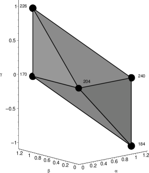
Figure 1: Visual representation of the set of all conservative PCA rules in the parameter space $(\alpha,\beta,\gamma)$.

5 Current conservation and fundamental diagrams

In [1], Hattori and Takesue demonstrated that existence of a conserved quantity in a deterministic CA is equivalent to a discrete version of a standard current conservation law $\partial\rho/\partial t=-\partial j/\partial x$. In what follows, we will show that a similar current conservation law holds for conservative PCA.

We will first observe that the sum on the right hand side of the condition (2) can be split into two parts, one depending on $x_{2},\ldots,x_{n}$, and another which depends on $x_{1},x_{2},\ldots,x_{n-1}$. We will therefore define the function of $n-1$ arguments

$$J(x_{1},x_{2},\ldots,x_{n-1})=-\sum_{k=1}^{n-1}f(\underbrace{0,0,\ldots,0}_{k},x_{1},x_{2},\ldots,x_{n-k})+\sum_{j=1}^{-c_{1}}x_{j},$$ (27)

With this definition, it is straightforward to show that

Proposition 4

A probabilistic CA rule $f$ is number-conserving if, and only if, for all $\{x_{1},x_{2},\ldots,x_{n}\}\in\{0,1\}^{n}$, it satisfies

$$f(x_{1},x_{2},\ldots,x_{n})-x_{-c_{1}+1}=J(x_{1},x_{2},\ldots,x_{n-1})-J(x_{2},x_{3},\ldots,x_{n}).$$ (28)

Applying this to all lattice sites we obtain

$$f(s_{i+c_{1}},s_{i+c_{2}},\ldots,s_{i+c_{n}})-s_{i}=J(s_{i+c_{1}},s_{i+c_{2}},\ldots,s_{i+c_{n-1}})\\ -J(s_{i+c_{2}},s_{i+c_{3}},\ldots,s_{i+c_{n-1}}),$$ (29)

where we dropped $k$ dependence for clarity.

In order to understand the full meaning of the above equation, let us recall a general formulation of a conservation law in a continuous, one dimensional physical system. Let $\rho(x,t)$ denote the density of some material at point $x$ and time $t$, and let $j(x,t)$ be the current (flux) of this material at point $x$ and time $t$. A conservation law states that the rate of change of the total amount of material contained in a fixed domain is equal to the flux of that material across the surface of the domain. The differential form of this condition can be written as

$$\frac{\partial\rho}{\partial t}=-\frac{\partial j}{\partial x}.$$ (30)

Interpreting $s_{i}(k)$ as the density, the left hand side of (29) is simply the expected change of density in a single time step, so that (29) is an obvious discrete analog of the current conservation law (30) with $J$ playing the role of the current. We can pursue this analogy even further. For the partial differential equation (30) one often assumes a functional relation between the current $j$ and the density $\rho$, and we will do the same for conservative PCA: we will ask how the “average” current $J$ depends on the “average” density in the stationary state, assuming that we start from a disordered initial condition.

To be more precise, let us now assume that the initial distribution $\mu$ is a Bernoulli distribution, i.e., at $k=0$, all sites $s_{i}(k)$ are independently occupied with probability $p$ or empty with probability $1-p$, where $p\in[0,1]$. Let us define $\rho(i,k)=E_{\mu}(s_{i}(k))$. Since the initial distribution is $i$-independent, we expect that $\rho(i,k)$ also does not depend on $i$, and we will therefore define $\rho(k)=\rho(i,k)$. Furthermore, for conservative PCA, $\rho(k)$ is $k$-independent, so we define $\rho=\rho(k)$. We will refer to $\rho$ as the density of occupied sites. The expected value of the current $J(s_{i+c_{1}}(k),s_{i+c_{2}}(k),\ldots,s_{i+c_{n-1}}(k))$ will also be $i$-independent, so we can define the expected current as

$$j(k,\rho)=E_{\mu}\big{(}J(s_{i+c_{1}}(k),s_{i+c_{2}}(k),\ldots,s_{i+c_{n-1}}(k))\big{)}.$$ (31)

The graph of the equilibrium current $j(\rho)=\lim_{k\rightarrow\infty}j(k,\rho)$ versus the density $\rho$ is known as the fundamental diagram. It has been numerically demonstrated [3] that for conservative deterministic CA the fundamental diagram usually develops a singularity as $k\rightarrow\infty$, meaning that $j(\rho)$ is not everywhere differentiable function of $\rho$.

6 Current and fundamental diagrams for nearest-neighbour PCA

For nearest-neighbour conservative PCA with the function $f$ given by eq. (26), the current becomes

$$J(x_{1},x_{2})=x_{1}-f(0,x_{1},x_{2})-f(0,0,x_{1})=\gamma x_{1}x_{2}+\alpha x_{1}-\beta x_{2},$$ (32)

and the conservation condition (28) becomes

$$f(x_{1},x_{2},x_{3})-x_{2}=J(x_{1},x_{2})-J(x_{2},x_{3}).$$ (33)

For the five nearest-neighbour deterministic rules, the current $J(x_{1},x_{2})$ assumes particularly simple form. For rule 184, the expression (32) reduces to $J(x_{1},x_{2})=x_{1}(1-x_{2})$, which means that the current $J(s_{i}(k),s_{i+1}(k))$ is non-zero only if $s_{i}(k)=1$ and $s_{i}(k)=0$. This agrees with the interpretation of rule 184 as a system of interacting particles, in which a particle located at site $i$ moves to site $i+1$ only if the site $i+1$ is empty. Rule $226$ is similar, except that particles move in the opposite direction than in the rule 184. For rules $240$, $170$ and $204$, the current becomes, respectively, $J(x_{1},x_{2})=x_{1}$, $J(x_{1},x_{2})=-x_{2}$, and $J(x_{1},x_{2})=0$. This means that all particles move to the right (rule 170), to the left (rule 240), or stay in the same place (rule 204).

It turns out that the simplicity of the expression for $J(x_{1},x_{2})$ for deterministic nearest-neighbour rules makes it possible to compute the expected current $j(k,\rho)$ exactly. For rule $204$, we obviously have $j(k,\rho)=0$. For rules $240$ and $170$ the expected current is just a linear function of $\rho$, and we have $j(k,\rho)=\rho$ for rule $240$ and $j(k,\rho)=-\rho$ for rule $170$.

For rule 184 (and its generalizations), one can also compute the expected current $j(k,\rho)$ exactly, as done in [11],

$$j(k,\rho)=1-\rho-\sum_{i=1}^{k+1}\frac{i}{k+1}\binom{2k+2}{k+1-i}\rho^{k+1-i}(1-\rho)^{k+1+i},$$ (34)

and one can prove that

$$j(\rho)=\lim_{k\rightarrow\infty}j(k,\rho)=-\left|\rho-\frac{1}{2}\right|+\frac{1}{2}.$$ (35)

This means that the graph of $j(\rho)$ versus $\rho$ has a singularity at $\rho=1/2$, as shown in Figure 2a. Rule $226$ exhibits similar behavior, except that the direction of the current is reversed.

Rule nr	$J(x_{1},x_{2})$	$j(k,\rho)$	$j(\rho)$
240	$x_{1}$	$\rho$	$\rho$
184	$x_{1}(1-x_{2})$	$\displaystyle 1-\rho-\sum_{i=1}^{k+1}\frac{i}{k+1}\binom{2k+2}{k+1-i}\rho^{k+1-i}(1-\rho)^{k+1+i}$	$\displaystyle-\left|\rho-\frac{1}{2}\right|+\frac{1}{2}$
204	$0$	$0$	$0$
226	$(1-x_{1})x_{2}$	$\displaystyle-1+\rho+\sum_{i=1}^{k+1}\frac{i}{k+1}\binom{2k+2}{k+1-i}\rho^{k+1-i}(1-\rho)^{k+1+i}$	$\displaystyle\left|\rho-\frac{1}{2}\right|-\frac{1}{2}$
170	$-x_{2}$	$-\rho$	$-\rho$

Table 2: Expected current $j(k,\rho)$ and the expected equilibrium current $j(\rho)$ for five deterministic elementary conservative CA.

Expressions for $j(k,\rho)$ and $j(\rho)$ for all five deterministic nearest-neighbour rules are summarized in Table 2. Unfortunately, these results cannot be easily generalized to compute expected currents for probabilistic rules. Even the equilibrium current $j(\rho)$ for the general rule given by eq. (26) does not seem to be analytically tractable, not to mention the time-dependent current $j(k,\rho)$. In the following section, we will use mean-field type technique to obtain approximate equilibrium current for probabilistic rules.

7 Mean Field Current

For nearest-neighbour rules, we can write the following expression for the average current, using equations (31) and (32),

$$j(k)=\gamma E_{\mu}\big{(}s_{i-1}(k)s_{i}(k)\big{)}+(\alpha-\beta)\rho,$$ (36)

where we used the fact that $E_{\mu}\big{(}s_{i}(k)\big{)}=\rho$. We will use abbreviated notation for probabilities $Pr(s_{i-1}(k),s_{i}(k)=a_{1}a_{2})$, denoting them simply by $P_{k}(a_{1}a_{2})$, where $a_{1},a_{2}\in\{0,1\}$. $P_{k}(11)$ is in this notation the probability that the pair $(s_{i-1}(k),s_{i}(k))$ is at time step $k$ in the state $(1,1)$, and since

$$E_{\mu}\big{(}s_{i-1}(k)s_{i}(k)\big{)}=Pr\big{(}(s_{i-1}(k),s_{i}(k))=(1,1)\big{)},$$ (37)

we obtain

$$j(k)=\gamma P_{k}(1,1)+(\alpha-\beta)\rho.$$ (38)

By (4), probabilities $P_{k}(a_{1}a_{2})$ must satisfy the following relationship

$$P_{k+1}(a_{1}a_{2})=\sum_{b_{1},b_{2},b_{3},b_{4}\in\{0,1\}}w(a_{1}a_{2}|b_{1}b_{2}b_{3}b_{4})P_{k}(b_{1}b_{2}b_{3}b_{4}),$$ (39)

where $w(a_{1}a_{2}|b_{1}b_{2}b_{3}b_{4})=w(a_{1}|b_{1}b_{2}b_{3})w(a_{2}|b_{2}b_{3}b_{4})$, and the values of transition probabilities $w$ are given by (22). As before, $P_{k}(b_{1}b_{2}b_{3}b_{4})$ is the probability that the sequence of four consecutive sites at time $k$ assumes value $(b_{1},b_{2},b_{3},b_{4})$.

The equation (39) gives two-site probabilities at time $k+1$ in terms of four-site probabilities at time $k$. In order to make it useful, we have to eliminate four-site probabilities from this equation. This can be done only approximately, using Bayesian extension formula also known as local structure theory [21],

$$P_{k}(b_{1}b_{2}b_{3}b_{4})\approx\frac{P_{k}(b_{1}b_{2})P_{k}(b_{2}b_{3})P_{k}(b_{3}b_{4})}{P_{k}(b_{2})P_{k}(b_{3})},$$ (40)

where $P_{k}(1)=\rho$, $P_{k}(0)=1-\rho$.

This approximation transforms (39) into a set of recurrence relations for pair probabilities $P_{k}(a_{1}a_{2})$. Fixed point of this set corresponds to the stationary state, and the knowledge of the fixed point value of $P_{k}(11)$ allows us to find $j(\rho)$ by (38).

Although computation of the aforementioned fixed point is too long and tedious to be attempted by hand, it can be carried out by a computer algebra software. The resulting stationary value of the current is shown below (we used “mf” subscript to indicate mean-field nature of the approximation (40)):

$$j_{\mathrm{mf}}(\rho)=(\alpha-\beta+\gamma)\rho-\frac{A\gamma\rho(\rho-1)}{2(\gamma\rho-\gamma+\beta)(-\gamma\rho+\gamma+\alpha)}$$ (41)

where

$$A=(\alpha-\beta+\gamma)(\alpha-\beta+\gamma-\gamma\rho)-\alpha-\beta+\alpha\beta$$

$$-{\rm sgn}(\gamma)\sqrt{c_{0}+c_{1}\rho+c_{2}\rho^{2}},$$ (42)

$$c_{{0}}={\beta}^{4}-2\left(2\gamma+1+\alpha\right){\beta}^{3}+\left(-5{\alpha}^{2}+4\gamma-4\gamma\alpha+1+2{\gamma}^{2}\right){\beta}^{2}$$

$$+2\left(\alpha-{\alpha}^{3}-{\gamma}^{2}+3\alpha{\gamma}^{2}+2\gamma{\alpha}^{2}\right)\beta-2\alpha{\gamma}^{2}-2{\alpha}^{3}$$

$$+4{\alpha}^{3}\gamma+{\gamma}^{4}+{\alpha}^{2}-4\gamma{\alpha}^{2}+{\alpha}^{4}+2{\gamma}^{2}{\alpha}^{2},$$ (43)

$$c_{{1}}=-2{\gamma}^{4}+2\left(\alpha-\beta\right){{\gamma}}^{3}+2\left(\alpha+\beta-{\alpha}^{2}-{\beta}^{2}-7\alpha\beta\right){\gamma}^{2}$$

$$+2\left({\beta}^{3}-{\alpha}^{3}+{\alpha}^{2}-{\beta}^{2}+2{\beta}^{2}\alpha-2{\alpha}^{2}\beta\right)\gamma$$ (44)

and

$$c_{{2}}={\gamma}^{2}\left({\alpha}^{2}+{\beta}^{2}+\gamma^{2}-2\gamma\alpha+6\alpha\beta+2\gamma\beta\right).$$ (45)

The above approximation does a remarkably good job in predicting $j(\rho)$ for deterministic rules. In fact, it yields all five expressions for the equilibrium current reported in the last column of Table 2.

For non-deterministic cases, the approximation does not work equally well. In order to evaluate its accuracy, we performed computer simulations in which the current $j(k,\rho)$ was recorded for large values of $k$, thus approximating the equilibrium current $j(\rho)$. Results are reported in Figure 2, where we show fundamental diagrams for a selection of five nearest-neighbour rules. Dotted lines represent simulation results, while continuous lines represent the approximate current given by (41). Values of parameters $\alpha$, $\beta$ and $\gamma$ are shown in the upper left corner of each diagram. Only one diagram, namely Figure 2a, corresponds to a deterministic rule (rule 184). All other diagrams represent non-deterministic rules.

Figure 2: Fundamental diagrams of selected nearest-neighbour conservative PCA rules. Horizontal axis represents the density $\rho$, while the vertical axis represents the stationary current $j(\rho)$. Solid dots represent simulation results, and the continuous lines are graphs of $j_{MF}(\rho)$ vs. $\rho$.

Diagram (b) correspond to the rule located on the edge of the polyhedron of Figure 1 joining rules 184 and 240, close to the vertex of rule $184$. Similarly, diagram (c) represents the rule located on the edge joining rules 184 and 170, again close to the vertex of rule $184$. Remarkably, it appears that the local structure theory predicts correctly the shape of the linear part of the fundamental diagram, while the nonlinear part is only approximately correct. It also predicts existence of the singularity in the fundamental diagram, while numerical simulations indicate that no such singularity exists.

When we consider a rule located on the edge joining rule 184 and rule 204, as shown in diagram (d), no part of the fundamental diagram is predicted correctly by the local structure theory (LST). The shape of the LST diagram, however, is not far from the observed shape. One can note similar phenomenon for a rule located on the base of the pyramid of Figure 1 (diagram e) or in the interior of the pyramid (diagram f).

The above evidence suggest some conjectures about fundamental diagrams of conservative PCA. First of all, singularity of the fundamental diagram appears to be a purely deterministic phenomenon. The fundamental diagram has a singularity (at $\rho=1/2$) only for rules 184 and 226. For all other rules, the graph of $j(\rho)$ has no “sharp corners”. Recall that the general probabilistic CA rule is defined in terms of probabilities $w(a|\mathbf{v})$. If all of these probabilities belong to the set $\{0,1\}$, such a rule will be called deterministic. All other PCA rules will be called truly probabilistic.

Conjecture 1

The equilibrium current $j(\rho)$ for any truly probabilistic conservative CA rule is a differentiable function of $\rho$ for $\rho\in(0,1)$.

Secondly, linear parts of fundamental diagrams can be computed exactly by using local structure approximation. This has been observed in [3] for deterministic rules, and appears to be true for probabilistic rules as well.

Conjecture 2

If the equilibrium current $j(\rho)$ of a probabilistic conservative CA rule is a linear function of $\rho$ in some interval $(a,b)\subseteq(0,1)$, then the local structure approximation for $j(\rho)$ in this interval is exact.

8 Conclusion

We have demonstrated that the concept of a conservation law can be naturally extended from deterministic to probabilistic cellular automata rules. Local function $f$ for conservative PCA must satisfy conditions analogous to conservation conditions for deterministic CA. We also proved that the local function must be 1-balanced. For nearest-neighbour rules, conservation conditions reduce the number of free parameters defining the rule to three, making it possible to visualize all nearest-neighbour rules as points of a polyhedron in 3D space, with deterministic rules located at vertices of the polyhedron.

Conservation condition for PCA can be also written as a current conservation law. For deterministic nearest-neighbour rules the current can be computed exactly, but for probabilistic rules it appears to be a much more difficult problem. Nevertheless, local structure approximation can partially predict the equilibrium current. For linear segments of the fundamental diagram it actually produces exact results.

Although our conjectures regarding fundamental diagrams are supported by numerical evidence for nearest-neighbour rules, obviously more evidence is needed, especially for larger neighbourhood sizes. Preliminary evidence indicates that both conjectures hold for four-input rules and five-input rules, and these findings will be reported elsewhere.

Another interesting question is the issue of representation. In [2], it has been demonstrated that conservative deterministic CA can be viewed as systems of interacting particles, or, in other words, that conservative CA rules can be defined using “motion representation” (as rules defining motion of individual particles). Similar concept has been introduced in [15] as a “displacement representation”. As pointed out in [22], the motion or displacement representation is analogous to Lagrange description of the fluid flow in hydrodynamics, in which we observe a particle and follow its trajectory. Standard definition of the CA rule (as in eq. 3), on the other hand, resembles Euler description of the flow, where the flow is observed at a fixed point in space and the dependent variable represents the amplitude of a field at that point. For deterministic conservative CA, both Langrange and Euler descriptions are possible. It seems that it should be possible to construct Lagrange description for probabilistic conservative CA as well, although it is not clear how to accomplish this task. The main problem is that the particles are not strictly conserved in PCA, only their expected number is. Since a given particle may disappear at any time, it is not possible to choose one particle and follow its trajectory indefinitely. Some averaging procedure will clearly be needed here.

Acknowledgements: The author acknowledges financial support from NSERC (Natural Sciences and Engineering Research Council of Canada) in the form of the Discovery Grant.

References

- [1] T. Hattori and S. Takesue, “Additive conserved quantities in discrete-time lattice dynamical systems,” Physica D 49 (1991) 295–322.
- [2] H. Fukś, “A class of cellular automata equivalent to deterministic particle systems,” in Hydrodynamic Limits and Related Topics, A. T. L. S. Feng and R. S. Varadhan, eds., Fields Institute Communications Series. AMS, Providence, RI, 2000. arXiv:nlin.CG/0207047.
- [3] N. Boccara and H. Fukś, “Cellular automaton rules conserving the number of active sites,” J. Phys. A: Math. Gen. 31 (1998) 6007–6018, arXiv:adap-org/9712003.
- [4] N. Boccara and H. Fukś, “Number-conserving cellular automaton rules,” Fundamenta Informaticae 52 (2002) 1–13, arXiv:adap-org/9905004.
- [5] H. Fukś and N. Boccara, “Convergence to equilibrium in a class of interacting particle systems,” Phys. Rev. E 64 (2001) 016117, arXiv:nlin.CG/0101037.
- [6] J. Krug and H. Spohn, “Universality classes for deterministic surface growth,” Phys. Rev. A 38 (1988) 4271–4283.
- [7] T. Nagatani, “Creation and annihilation of traffic jams in a stochastic assymetric exclusion model with open boundaries: a computer simulation,” J. Phys. A: Math. Gen. 28 (1999) 7079–7088.
- [8] K. Nagel, “Particle hopping models and traffic flow theory,” Phys. Rev. E 53 (1996) 4655–4672, arXiv:cond-mat/9509075.
- [9] V. Belitsky and P. A. Ferrari, “Invariant measures and convergence for cellular automaton 184 and related processes,” math.PR/9811103. Preprint.
- [10] M. S. Capcarrere, M. Sipper, and M. Tomassini, “Two-state, r=1 cellular automaton that classifies density,” Phys. Rev. Lett. 77 (1996) 4969–4971.
- [11] H. Fukś, “Exact results for deterministic cellular automata traffic models,” Phys. Rev. E 60 (1999) 197–202, arXiv:comp-gas/9902001.
- [12] K. Nishinari and D. Takahashi, “Analytical properties of ultradiscrete burgers equation and rule-184 cellular automaton,” J. Phys. A-Math. Gen. 31 (1998) 5439–5450.
- [13] V. Belitsky, J. Krug, E. J. Neves, and G. M. Schutz, “A cellular automaton model for two-lane traffic,” J. Stat. Phys. 103 (2001) 945–971.
- [14] M. Blank, “Ergodic properties of a simple deterministic traffic flow model,” J. Stat. Phys. 111 (2003) 903–930.
- [15] M. Pivato, “Conservation laws in cellular automata,” Nonlinearity 15 (2002) 1781–1793, arXiv:math.DS/0111014.
- [16] A. Moreira, “Universality and decidability of number-conserving cellular automata,” Theor. Comput. Sci. 292 (2003) 711–721.
- [17] J. V. Kujala and T. J. Lukka, “Solutions for certain number-conserving deterministic cellular automata,” Phys. Rev. E 65 (2002) art. no.–026115.
- [18] H. Fukś, “Non-deterministic density classification with diffusive probabilistic cellular automata,” Phys. Rev. E 66 (2002) 066106, arXiv:nlin.CG/0302015.
- [19] N. G. de Bruijn, “A combinatorial problem,” Nederl. Akad. Wetensch. Proc. 49 (1946) 758–746.
- [20] A. Ralston, “De Bruijn sequences – a model example of the interaction of discrete mathematics and computer science,” Math. Mag. 55 (1982) 131–143.
- [21] H. A. Gutowitz, J. D. Victor, and B. W. Knight, “Local structure theory for cellular automata,” Physica D 28 (1987) 18–48.
- [22] J. Matsukidaira and K. Nishinari, “Euler-Lagrange correspondence of cellular automaton for traffic-flow models,” Phys. Rev. Lett. 90 (2003) art. no.–088701.