A frequency measure robust to linear filtering

Abstract

A definition of frequency (cycles per unit-time) based on an approximate reconstruction of the phase-space trajectory of an oscillator from a signal is introduced. It is shown to be invariant under linear filtering, and therefore inaccessible by spectral methods. The effect of filtering on frequency in cases where this definition does not perfectly apply is quantified.

1 Introduction

In the experimental exploration of complex systems, such es those encountered in life-science, geology, or astronomy, it is not unusual that the experimenter discovers oscillations of unknown origin in a measured time-series. The experimenter would then usually try to characterize these oscillations in a form that admits an identification of their source – the oscillator. The conventional first choice is a characterization of the oscillations by their “frequency”. For an ideal, periodically oscillating signal $x(t)$, the smallest number $T>0$ such that $x(t)=x(t+T)$ for all $t$ is the period of the signal, and its (angular) frequency is defined by $\omega=2\pi/T$. There is a good reason for choosing this particular characterization. All other properties of an ideal, periodic signal, i.e. its waveform and amplitude, are subject to distortions along the signal pathway from the oscillator to the detector. In fact, linear filtering along the signal pathway would generally be sufficient to modify the waveform and the amplitude in an arbitrary way. And the precise properties of the signal pathway are unknown in the setting considered here. The frequency information is the only sure fact. For ideal, periodic oscillations, these observations are too obvious to deserve much discussion. But for non-ideal oscillations, as they are frequently encountered in complex systems, the situation is less clear.

A large variety of methods is being used to determine a “frequency” for non-ideal oscillations, and not all of them are equally robust to filtering and other distortions. Two major kinds of methods can be distinguished: Firstly, there are period-counting methods, where, from the number of oscillation periods $n(\Delta t)$ in a time interval $[t_{0},t_{0}+\Delta t]$, the frequency is determined as

$$\omega_{\rm{count}}=\lim_{\Delta t\to\infty}\frac{2\pi n(\Delta t)}{\Delta t}.$$ (1)

(Finite sample-size effects are not discussed here.) The methods differ in the criteria used for counting individual periods (e.g., local maxima, zero-crossings). Secondly, there are spectral methods, where the frequency $\omega_{\rm{spec}}$ characterizes the position of a peak in an estimate of the power spectral density $S_{x}(\omega)$ [1, 2] of the signal $x(t)$ (e.g., [3, 4, 5, 6, 7]). Often, the frequency with maximum power $\omega_{\rm{peak}}$ is used. The term spectral methods shall here also include methods based on estimates of the autocorrelation function of the signal, since this is related to the spectral density by a simple Fourier transformation.

For weak distortions and not too irregular oscillations, period-counting methods can be just as unequivocal as frequency measurements for ideal oscillations. This is why they are routinely used in high-precision frequency (or time) measurements. They are also naturally associated with mode-locking phenomena [8]. But for stronger distortions and more irregular oscillations, this robustness is reverted to its contrary. Unequivocally identifying individual periods of oscillation then becomes difficult. In these situations spectral methods are generally preferred. However, it is obvious that spectral methods are not robust to filtering along the signal pathway either. By linear filtering, the power spectrum can be modified nearly arbitrarily.

How much can the concept of period-counting frequency measurement be extended to distorted time series? A partial answer is given in this work. In section 2.1 a generalized period-counting frequency measure, the topological frequency, is defined. It is based on the approximate reconstruction of the phase-space trajectory of the oscillator. In section 2.2 it is shown that the topological frequency is robust with respect to nearly arbitrary linear filtering. This has three important implications: (i) At least as long as the signal pathway acts as a linear filter, the topological frequency is a characteristic of the (typically nonlinear) oscillator alone. (ii) Filtering of the signal, in order to remove noise and other undesirable components, does no harm to the result for the frequency. In view of (i) and (ii), the topological frequency can be considered to be robust with respect to both kinds of distortions, filtering and noise. Finally, (iii) the results of frequency measurements using spectral methods can deviate arbitrarily from the topological frequency. This point is made rigorous in section 2.3.

Not for all oscillatory time series can the topological frequency be defined. In particular, linear time series driven by Gaussian noise are excluded. Weakly nonlinear models for noisy time series can interpolate between linear Gaussian oscillations and ideal periodicity. For these models, the influence of filtering on a weaker period-counting frequency measure, the average or phase frequency (see below), is investigated in section 3. The susceptibility of the phase frequency to filtering is found to decay rapidly with the degree of nonlinearity. Section 4 contains some concluding remarks.

2 Topological Frequency

2.1 Definitions

The theory becomes more transparent in a discrete-time representation. Let $\{x_{t}\}$ be an infinite, real-valued time series sampled at equally spaced times starting at $t=0$. Measure time in units of the sampling interval. Define the spectral density $S_{x}(\omega)$ of $\{x_{t}\}$ as

$$S_{x}(\omega)=\frac{1}{2\pi}\sum_{\tau=-\infty}^{\infty}\left<x_{t}\,x_{t+|\tau|}\right>_{t}\cos({\omega\tau}),$$ (2)

where $\left<\cdot\right>_{t}$ denotes temporal averaging ($t\geq 0$).

Let the trajectory $p(t)$ of a time series $\{x_{t}\}$ in $N$-dimensional delay space be defined by $p(t)=(x_{t},x_{t-1},\ldots,x_{t-N+1})$ for integer $t$ and by linear interpolation for non-integer $t$. Frequency will here be defined with respect to a Poincaré section or counter, which is an $(N-1)$-dimensional, oriented manifold $M$ with boundary $\partial M$ and interior $\mathop{\mathrm{Int}}M=M\backslash\partial M$, embedded in the $N$-dimensional delay space.

Let $n(t_{1})$ be the oriented number of transitions of the trajectory $p(t)$ through $\mathop{\mathrm{Int}}M$ in the time interval $0<t<t_{1}$. That is, a transition through $\mathop{\mathrm{Int}}M$ in positive (negative) direction increments (decrements) $n(t_{1})$ by one. For example, a positive-slope zero-crossing counter in $2$-dimensional delay space would be given by

$$M=\{(v_{1},v_{2})\in\mathbb{R}^{2}|v_{1}+v_{2}=0,\,v_{1}\geq v_{2}\}.$$ (3)

Define the topological frequency $\omega_{M,x}$ of $\{x_{t}\}$ with respect to a counter $M$, as

$$\omega_{M,x}:=\lim_{t\to\infty}\frac{2\pi|n(t)|}{t},$$ (4)

provided the limit exists and there is a $d>0$ such that $p(t)$ has for all $t\geq 0$ a distance $>d$ from $\partial M$. By construction, $\omega_{M,x}$ is invariant under not too large deformations of $\{x_{t}\}$ and $M$. For example, if the trajectory contains a loop which comes close to $\mathop{\mathrm{Int}}M$ but does not encircle $\partial M$, a small deformation of $\{x_{t}\}$ or $M$ might make the loop intersect $\mathop{\mathrm{Int}}M$. But, since this intersection comprises two transitions of the trajectory through $\mathop{\mathrm{Int}}M$, one of which is positive and one of which is negative, the value of $n(t)$ does not change for large enough $t$. Configurations with $p(t)$ tangential to $\mathop{\mathrm{Int}}M$ can be evaluated as either of both limiting cases – intersecting or not – without effecting $\omega_{M,x}$. Drastically different counters can lead to different frequencies. But each of these is sharply defined.

2.2 Invariance under filtering

It can be shown that for any bounded time series $\{x_{t}\}$ the topological frequency is invariant under nearly arbitrary linear filtering:

Theorem 1. Let $\{y_{t}\}$ be obtained from a bounded time series $\{x_{t}\}$ by linear, causal filtering,

$$y_{t}:=\sum_{k=0}^{\infty}a_{k}\,x_{t-k}.$$ (5)

Assume that, for some $r>1$,

$$0<\left|\sum_{k=0}^{\infty}a_{k}\,z^{k}\right|<\infty$$ (6)

for all complex $z$, $r^{-1}<|z|<r$. (This excludes, for example, filters which fully block some frequencies.) Let $M$ be a counter and $\omega_{M,x}$ be defined. Then there is, at sufficiently high embedding dimension, a counter $M^{\prime}$ such that $\omega_{M^{\prime},y}$ is defined and $\omega_{M^{\prime},y}=\omega_{M,x}$.

Proof. This is most easily seen by the following explicit construction of an appropriate counter $M^{\prime}$: Notice that the filter $\{a_{k}\}$ has a (not necessarily causal) inverse $\{b_{j}\}$ given by

$$\sum_{j=-\infty}^{\infty}b_{j}\,z^{j}:=\left(\sum_{k=0}^{\infty}a_{k}\,z^{k}\right)^{-1},$$ (7)

$r^{-1}<|z|<r$. Let $C$ be an upper bound for $|x_{t}|$ and $d$ be the (minimum) distance of the trajectory of $\{x_{t}\}$ from $\partial M$ in the maximum norm. For notational convenience define $x_{t}=y_{t}=0$ for $t<0$. Let

$$u_{t}:=\sum_{j=-L}^{L}b_{j}y_{t-j},$$ (8)

where $L$ is chosen such that

$$|x_{t}-u_{t}|=\left|\left(\sum_{j=-\infty}^{-L-1}+\sum_{j=L+1}^{\infty}\right)\sum_{k=0}^{\infty}b_{j}a_{k}x_{t-j-k}\right|$$

$$\hbox to0.0pt{\hss${}<{}$}\left(\sum_{j=L+1}^{\infty}|b_{j}|+|b_{-j}|\right)\left(\sum_{k=-\infty}^{\infty}|a_{k}|\right)\,C$$

$$\hbox to0.0pt{\hss${}\leq{}$}d/2$$ (9)

for all integer $t$. Convergence of the left hand side of (7) guarantees that such an $L$ exists. $\{u_{t}\}$ is an approximation of $\{x_{t}\}$ reconstructed from $\{y_{t}\}$ using the filter (8). Since the approximation error of the time series is at most $d/2$, so is, in the maximum norm, the approximation error of the trajectory. In particular, the topological relation between the trajectory and the counter $M$ is not changed by going over from $\{x_{t}\}$ to $\{u_{t}\}$ (except for some pairs of forward/backward transitions through $M$, which do not contribute to the limit (4)). Hence, $\omega_{M,u}=\omega_{M,x}$.

Now, notice that the $N$-dimensional delay embedding of $\{u_{t}\}$ can be obtained by a linear projection

$$(u_{t},\ldots,u_{t-(N-1)})^{T}\!\!=\mathbf{P}\,(y_{t+L},\ldots,y_{t-(L+N-1)})^{T}$$ (10)

from the $2L+N$-dimensional delay embedding of $\{y_{t}\}$ [9, 10], with the matrix elements of $\mathbf{P}$ given by (8). Furthermore, $\mathbf{P}$ maps the trajectory of $\{y_{t+L}\}$ onto the trajectory of $\{u_{t}\}$. Define the oriented manifold $M^{\prime}$ such that

$$\mathbf{v}\in M^{\prime}\Leftrightarrow\mathbf{P}\mathbf{v}\in M\quad(\mathbf{v}\in\mathbb{R}^{2L+N})$$ (11)

and $\partial M=\mathbf{P}\partial M^{\prime}$ in the obvious way. This guarantees a finite distance of the trajectory of $\{y_{t}\}$ from $\partial M^{\prime}$, and there is a one-to-one correspondence between transitions of the trajectory of $\{u_{t}\}$ through $M$ and transitions of the trajectory of $\{y_{t}\}$ through $M^{\prime}$. Hence, $\omega_{M^{\prime},y}=\omega_{M,u}=\omega_{M,x}$, proving Theorem 1. $\square$

2.3 The arbitrariness of the power spectrum, given the topological frequency

Spectral frequency measures depend on the time series through the power spectral density $S(\omega)$ alone. By showing that $S(\omega)$ is independent of the topological frequency, it becomes clear that spectral frequency measures can generally differ arbitrarily from the topological frequency, in contrast to what one might intuitively assume (see, e.g., reference [11], p 226).

Theorem 2. Let $S_{0}(\omega)\geq 0$ ($\omega\in[-\pi,\pi]$) be a symmetric, continuous function, $0<\omega_{0}<\pi$ and $\epsilon>0$. Then there is a time series $\{y_{t}\}$, an embedding dimension $N$ and a counter $M\subset\mathbb{R}^{N}$ such that $\omega_{M,y}=\omega_{0}$ and

$$\left|S_{y}(\omega)-S_{0}(\omega)\right|<\epsilon\quad\hbox{for all $\omega\in[-\pi,\pi]$},$$ (12)

where $S_{y}(\omega)$ is the power spectral density of $\{y_{t}\}$.

Proof. In order to obtain $\{y_{t}\}$ as described in Theorem 2, take a time series $\{x_{t}\}$ which oscillates with frequency $\omega_{0}$ and adjust the spectral density by filtering. A suitable time series to start with is given by

$$x_{t}=2\cos(i\,\omega_{0}\,t+i\,\phi_{t})\rm{\ with\ }\phi_{0}=0\rm{\ and\ }\phi_{t+1}=\phi_{t}+\vartheta\,\epsilon_{t},$$ (13)

where $\{\epsilon_{t}\}$ is an equally distributed random sequence of the values $-1$ and $1$. With the counter $M$ given by (3), the topological frequency $\omega_{M,x}=\omega_{0}$ is defined when

$$0<\vartheta<\left\{\begin{array}[]{ll}\omega_{0}&\hbox{for}\quad 0<\omega_{0}<\pi/2,\\ \arcsin(\sin^{2}\!\omega_{0})&\hbox{for}\quad\pi/2\leq\omega_{0}<\pi.\\ \end{array}\right.$$ (14)

The autocorrelation function of $\{x_{t}\}$ is $\left<x_{t}\,x_{t+\tau}\right>_{t}=2\,(\cos\vartheta)^{\tau}\cos\omega_{0}\tau$ and its spectral density

$$S_{x}(\omega)=\frac{\sin^{2}\!\vartheta\,\left(1+\cos^{2}\!\vartheta-2\cos\vartheta\,\cos\omega\,\cos\omega_{0}\right)}{\pi\left|1-e^{i(\omega-\omega_{0})}\cos\vartheta\right|^{2}\left|1-e^{i(\omega+\omega_{0})}\cos\vartheta\right|^{2}}$$ (15)

is positive and continuous as required below. In order to see that there is a suitable set of filter coefficients $\{a_{k}\}$, notice that, as an immediate consequence of Theorem 4.4.3 of reference [1], there is, for any $\epsilon>0$ and any two continuous, symmetric spectral densities $S_{x}(\omega)>0$ and $S_{0}(\omega)$ ($\omega\in[-\pi,\pi]$), a non-negative integer $p$ and a polynomial $c(z)=1+c_{1}z+\ldots+c_{p}z^{p}$ such that

$$c(z)\neq 0\quad\hbox{for $|z|\leq 1$}$$ (16)

and, for all $\omega\in[-\pi,\pi]$,

$$\left|C\left|c(e^{-i\omega})\right|^{2}-\frac{S(\omega)}{S_{x}(\omega)}\right|<\frac{\epsilon}{\max_{\lambda}S_{x}(\lambda)},$$ (17)

where $C=(1+c_{1}^{2}+\ldots+c_{p}^{2})^{-1}\pi^{-1}\int^{\pi}_{0}S(\omega)/S_{x}(\omega)\,d\omega$. Setting $a(z)=C^{1/2}c(z)$, $a_{0}=C^{1/2}$, $a_{k}=C^{1/2}c_{k}$ ($k=1,\ldots,p$), and all other $a_{k}=0$, $\{y_{t}\}$ given by (5) has the spectral density $S_{y}(\omega)=|a(e^{-i\omega})|^{2}S_{x}(\omega)$ (see, e.g., reference [1], Theorem 4.4.1) and inequality (17) implies (12). By (16) the filter $\{a_{k}\}$ satisfies the invertibility condition (6) of Theorem 1. Thus, an appropriate counter $M$ can be obtained such that $\omega_{M,y}=\omega_{0}$ and Theorem 2 is proven. It should be mentioned that when $S_{0}(\omega)$ is analytic for real $\omega$, Theorem 2 generally holds also with the perfect identity $S_{y}(\omega)=S_{0}(\omega)$ instead of inequality (12). $\square$

2.4 An Example

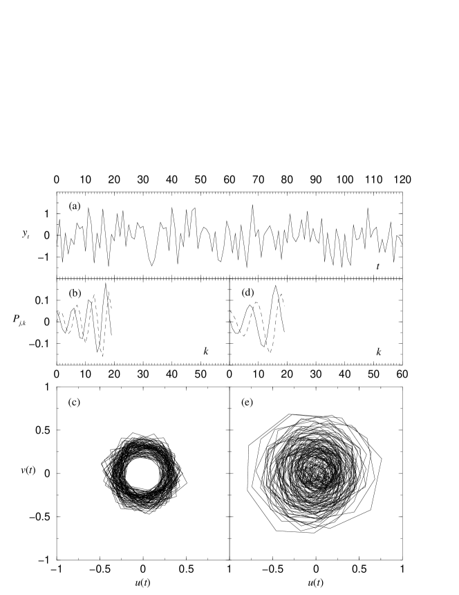
Figure 1: Demonstration for Theorem 2. (a) A representative segment of the white-noise time series ${y_{t}}$ introduced in section 2.4, (b) the components $P_{1,k}$ (solid) and $P_{2,k}$ (dashed) of a projector from its 20D delay embedding to 2D, and (c) a segment of the projected trajectory $p(t)$ of ${y_{t}}$, with $(u(t),v(t))^{T}:=\mathbf{P}p(t)$. The frequency can be read off. Alternatively (d) another, inappropriate projector, and (e) the projected trajectory.

As a demonstration for Theorem 2, consider the time series $\{y_{t}\}$ shown in figure 1a. By construction, it is a realization of a white-noise process. It was obtained by “bleaching” [12] a realization of $\{x_{t}\}$ given by (13) with $\omega_{0}=1.1$ and $\theta=0.4$, i.e., the realization was filtered such as to transform the known spectral density (15) into a white spectrum. Although all spectral information was lost, $\omega_{0}$ can precisely be recovered from $\{y_{t}\}$. Using an automated search algorithm (to be described elsewhere), a projection matrix $\mathbf{P}$ (figure 1b) is found, such that the projection of the 20D embedding of $\{y_{t}\}$ into 2D yields a trajectory with a nice circular structure and a “hole” in the center (figure 1c). The number of oscillations and the frequency are obvious; $\omega_{0}$ is recovered. Any line extending from the origin to infinity can serve as a counter $M$ in the 2D projection. This can be used to obtain a corresponding counter $M^{\prime}$ in 20D by a back-projection as in (11).

A projection with an inadequate $\mathbf{P}$ would not yield a different frequency, but only a criss-cross kind of trajectory (figure 1d,e), typically with an approximately Gaussian distribution of values with a maximum density at the origin. From such a representation, no positive topological frequency can be obtained.

The two-step procedure used here to obtain the counter $M^{\prime}$ via a counter $M$ in 2D works for many experimental time series, even though the concept of topological frequency is more general. The projector $\mathbf{P}$ can then be interpreted as a complex-valued filter $\{f_{k}\}$ with the impulse response function $f_{k}=P_{1,k}+i\,P_{2,k}$. In section 3.3 we come back to this point.

3 Noisy, weakly nonlinear oscillations

There are two assumptions upon which Theorem 1 is based – the boundedness of $\{x_{t}\}$ and the finite distance of its trajectory from $\partial M$ – which are not perfectly satisfied by typical noisy processes. Rather, the probability of reaching some point in delay space decreases exponentially (or faster) with the distance from some “average” trajectory and the inverse noise strength. For many processes the two assumptions and, as a consequence, the invariance of the $\omega_{\rm{count}}$ under filtering hold therefore only up to an exponentially small error. For signals generated by noisy, weakly nonlinear oscillators, an analytic estimate of this error shall now be derived.

Due to the separation of time scales inherent in the weakly nonlinear limit, it is more appropriate to work in a continuous-time representation. Consider the noisy, weakly nonlinear oscillator described by a complex amplitude $A(t)$ with dynamics given by the noisy Landau-Stuart equation [13]

$$\dot{A}=(\epsilon+i\omega_{0})A-(1+ig_{i})|A|^{2}A+\eta(t),$$ (18)

where $\epsilon$, $\omega_{0}$, and $g_{i}$ are real and $\eta(t)$ denotes complex, white noise with correlations

$$\left<\eta(t)\eta(t^{\prime})\right>=0,\quad\left<\eta(t)\eta(t^{\prime})^{*}\right>=4\delta(t-t^{\prime})$$ (19)

[^∗ $\equiv$ complex conjugation, $\left<\cdot\right>$ $\equiv$ expectation value]. In a certain sense, this system universally describes noisy oscillations in the vicinity of a Hopf bifurcation [14].

3.1 Definitions of frequency

Figure 2: The power spectrum $S_{A}(\omega)$ of $A(t)$ given by equations (18,19) with $\epsilon=2$ and $g_{i}=1$, obtained from a numerical simulation; and $\omega_{\rm{peak},A}$ (analytic results in reference [15]), compared to the mean frequency $\omega_{\rm{mean},A}=\omega_{0}-g_{i}\left<|A|^{4}\!\right>/\left<|A|^{2}\!\right>$ [$\left<|A|^{2n}\!\right>=2^{n}\,\mathcal{N}^{-1}\,d^{n}\!\mathcal{N}/d\epsilon^{n}$, see (28)] and the phase frequency $\omega_{\rm{ph},A}=\omega_{0}-g_{i}\left<|A|^{2}\!\right>$, defined by equations (20,21), and the linear frequency $\omega_{0}$.

For the reasons explained above, the topological frequency cannot be defined rigorously for noisy, weakly nonlinear oscillators. The customary frequency measures, such as the linear frequency $\omega_{0}$, the spectral peak frequency $\omega_{\rm{peak}}$, the average frequency or phase frequency

$$\omega_{\rm{ph},A}:=\left<\omega_{i}\right>,\quad\omega_{i}:=\mathrm{Im}\left\{\smash{[}t]{\dot{A}}/A\right\},$$ (20)

and the mean frequency

$$\omega_{\rm{mean},A}:=\frac{\left<\omega_{i}|A|^{2}\right>}{\left<|A|^{2}\right>}=\frac{\mathrm{Im}\left<\smash{\dot{A}}A^{*}\right>}{\left<|A|^{2}\right>}=\frac{\int\omega S_{A}(\omega)d\omega}{\int S_{A}(\omega)d\omega}$$ (21)

will generally (i.e., with $g_{i}\neq 0$) all yield different values; see figure 2. [Definitions (20,21) are sometimes restricted to “analytic signals” ($S_{A}(\omega)=0$ for $\omega<0$) derived from the corresponding real-valued signals $\mathrm{Re}\{A(t)\}$. See reference [16] for the history.]

The phase frequency measures the average number of circulations around the point $A=0$ in phase space per unit time (decompose $A(t)=a(t)e^{i\phi(t)}$ to see this). It is a period-counting frequency and the quantity which comes conceptually closest to the topological frequency. However, the choice of the point $A=0$ can here be justified only by symmetry and dynamics [the invariant density pertaining to equation (18) has an extremum at $A=0$], and not by invariance under perturbations. $\omega_{\rm{peak}}$ and $\omega_{\rm{mean}}$ are both spectral frequency measures, and the influence of filtering is obvious. But how does filtering affect $\omega_{\rm{ph},A}$? The following considerations lead to a surprisingly accurate result.

3.2 The effect of filtering on the phase frequency

The dynamics of $A$ on short time scales $\delta t$ is dominated by the driving noise, and the change in $A$ is of the order $|\delta A|=\mathcal{O}(4\delta t)^{1/2}$. A band-pass filter of spectral width $\Delta\omega$ which truncates the tails of the peak corresponding to $A$ in the power spectrum suppresses this diffusive motion on time scales $\Delta\omega^{-1}$, while on longer time scales dynamics change only little. The corresponding deformation of the path of $A$ in the complex plane can alter the number of circulations of the origin whenever $A$ approaches the origin to less then $\approx(4/\Delta\omega)^{1/2}$. At these times $|A|$ is small and, for not too narrow filters, the dynamics of $A$ in its linear range. Thus, the effect of broad-band filtering can be estimated by a linear theory. Consider, for a moment, the linearized version of equation (18),

$$\dot{A}=(\epsilon+i\omega_{0})A+\eta(t),$$ (22)

with $\eta(t)$ as above, and assume $\epsilon<0$. Clearly, $\omega_{\rm{ph},A}=\omega_{0}$. For the phase frequency of a complex, Gaussian, linear process $B(t)$ in general, a simple calculation shows $\omega_{\rm{ph},B}=\omega_{\rm{mean},B}$. This can be used to calculate the phase frequencies of $A$ after filtering. Let, for example, $B$ be obtained from $A$ through the primitive band-pass filter

$$\dot{B}=(-\epsilon_{1}+i\omega_{1})B+A,$$ (23)

which is centered at $\omega_{1}$ with width $\epsilon_{1}>0$. Using $\omega_{\rm{ph},B}=\omega_{\rm{mean},B}$ and elementary filter theory [2] one obtains

$$\omega_{\rm{ph},B}=\frac{\epsilon_{1}\,\omega_{0}-\epsilon\,\omega_{1}}{\epsilon_{1}-\epsilon}.$$ (24)

Table 1: The shift $\delta\omega_{\rm{num}}$ in the phase frequency $\omega_{\rm{ph},A}$ of $A(t)$, obtained from simulations of equations (18,19) with $g_{i}=1$, after filtering as in (23), and a comparison with the theoretical estimate (29). The data verify $\delta\omega\sim\epsilon_{1}^{-1}$, $\sim(\omega_{1}-\omega_{0})$, and $\sim\mathcal{N}^{-1}$ in this order.

• $\epsilon$	$(\omega_{\rm{ph},A}-\omega_{0})$	$(\omega_{1}-\omega_{0})$	$\epsilon_{1}$	$\delta\omega_{\rm{theo}}$	$\delta\omega_{\rm{num}}$
  2	$-2.2253$	$-2.5$	48	$-0.0117$	$-0.0109(16)$
  2	$-2.2253$	$-2.5$	24	$-0.0235$	$-0.0228(16)$
  2	$-2.2253$	$-2.5$	12	$-0.0469$	$-0.0437(15)$
  2	$-2.2253$	$\phantom{-}0.0$	24	$\phantom{-}0.0000$	$\phantom{-}0.0003(17)$
  2	$-2.2253$	$\phantom{-}2.5$	24	$\phantom{-}0.0235$	$\phantom{-}0.0226(16)$
  0	$-1.1284$	$-2.5$	24	$-0.1175$	$-0.1036(47)$
  3	$-3.0605$	$-2.5$	24	$-0.0063$	$-0.0074(13)$
  4	$-4.0104$	$-2.5$	24	$-0.0011$	$-0.0012(11)$

By the argument given above, the shift in phase frequency $\delta\omega:=\omega_{\rm{ph},B}-\omega_{\rm{ph},A}=(\omega_{0}-\omega_{1})\,(\epsilon/\epsilon_{1})+\mathcal{O}(\epsilon_{1}^{-2})$ is due to the times where $|A|^{2}\lesssim 4/\epsilon_{1}$. Since $A$ has a complex normal distribution with variance $\big{<}|A|^{2}\big{>}=-1/\epsilon$, this happens about

$$p\left[|A|^{2}<\frac{4}{\epsilon_{1}}\right]=1-\exp\left(\frac{2\epsilon}{\epsilon_{1}}\right)=-\frac{2\epsilon}{\epsilon_{1}}+\mathcal{O}(\epsilon_{1}^{-2})$$ (25)

of all times. Thus, during these times, the shift in phase frequency is $\delta\omega/p[|A|^{2}<{4}/{\epsilon_{1}}]=(\omega_{1}-\omega_{0})/2+\mathcal{O}(\epsilon_{1}^{-2})$. Extrapolation to $\epsilon>0$ and the weakly nonlinear case yields

$$\delta\omega=p\left[|A|^{2}<\frac{4}{\epsilon_{1}}\right]\frac{\omega_{1}-\omega_{0}}{2}+\mathcal{O}(\epsilon_{1}^{-2}),$$ (26)

now with

$$p[|A|^{2}<I_{0}]=\frac{1}{\mathcal{N}}\int_{0}^{I_{0}}\exp\left(\displaystyle\frac{\epsilon I}{2}-\frac{I^{2}}{4}\right)\,dI=\frac{I_{0}}{\mathcal{N}}+\mathcal{O}(I_{0}^{2}),$$ (27)

where

$$\mathcal{N}=\pi^{1/2}\exp(\epsilon^{2}/4)[1+\mathop{\rm{erf}}(\epsilon/2)].$$ (28)

Equations (26-28) predict the shift

$$\delta\omega=2\epsilon_{1}^{-1}\mathcal{N}^{-1}(\omega_{1}-\omega_{0})+\mathcal{O}(\epsilon_{1}^{-2})$$ (29)

in the phase frequency of $A(t)$ given by (18,19) after passing through the filter (23). A numerical test verifying this result is shown in table 1; notice in particular the fast decay of $\delta\omega$ as $\epsilon$ increases [$\delta\omega\sim\exp(-4/\epsilon^{2})$] and the conditions of Theorem 1 are better satisfied. The high accuracy of the result might be understood by observing that the crude upper bound $|A|^{2}<{4}/{\epsilon_{1}}$ enters the derivation of (29) two times, its numerical value canceling out.

3.3 The frequency of real-valued, weakly nonlinear signals

Experimental signals are real-valued. Assume that, instead of $A(t)$, only a real-valued signal $x(t)=\mathrm{Re}\{A(t)+(\hbox{higher harmonics})\}+(\hbox{perturbations})$ is given. The natural way to estimate the phase frequency of $A(t)$ then is to construct an approximation $\hat{A}(t)=(f*x)(t)$ of $A(t)$ by a convolution of $x(t)$ with a complex-valued filter $f(t)$, and to estimate the phase frequency as $\hat{\omega}_{\rm{ph},A}=\omega_{\rm{ph},\hat{A}}$. The filter $f(t)$ describes the combined effect of 2D delay embedding or analytic-signal construction, and filtering to eliminate higher harmonics, offsets, aliasing, and external perturbations. The result above shows that generally, for $\hat{\omega}_{\rm{ph},A}$ to be unbiased, the total effect of all these transformations should be a complex, symmetric band-pass centered on the linear frequency $\omega_{0}$ ($\neq\omega_{\rm{ph}},\,\omega_{\rm{peak}}$!). Otherwise there is a bias which decays as $\exp(-4/\epsilon^{2})$ for large $\epsilon$. To the extent that the bias vanishes, the probability of finding values of $\hat{A}(t)\approx A(t)\approx 0$ vanishes, too. Then, a counter $M^{\prime}$ for $x(t)$ can be obtained along the lines of section 2.4 using the filter $f(t)$ – approximated by a time-discrete filter $f_{k}$ – for the projection to 2D. Obviously, the corresponding topological frequency $\omega_{M^{\prime},x}$ equals $\hat{\omega}_{\rm{ph},A}$.

4 Conclusion

When the spectral density is of genuine interest, forget period counting. But there are many real-world applications (e.g.,  in astronomy [3], earth science [4], biomedicine [6, 5], or engineering [7]) where neither the characteristics of the signal pathway nor a detailed model of the oscillator are known, and yet a robust measure of the frequency or, at least, some robust characterization of the oscillator is sought. Then, by Theorem 2, spectral methods miss valuable information. In view of Theorem 1 and equation (29), concepts such as topological frequency or its little brother, phase frequency, are more appropriate. The fractal dimension of the reconstructed attractors, an alternative characterization, is typically robust with respect to finite-impulse-response filtering only [9, 10], i.e., only if there is a $q$ such that $a_{k}=0$ for $k>q$ in (5).

For a practical application of topological frequency, a systematic method to find appropriate counters in the typically high-dimensional delay spaces is desirable. Some progress in this direction has be made and will be reported elsewhere.

References

- [1] Brockwell P and Davis R 1991 Time Series: Theory and Methods Springer Series in Statistics (New York: Springer) 2nd edn.
- [2] Priestley M 1981 Spectral analysis and time series (London: Academic Press)
- [3] Méndez M et al. 1998 Difference frequency of kilohertz QPOS not equal to half the burst oscillation frequency in 4U 1636-53 Astrophys. J. 506 L117–L119
- [4] Godano C and Capuano P 1999 Source characterisation of low frequency events at stromboli and vulcano islands (isole eolie italy) J. Seismol. 3(4) 393–408
- [5] Korhonen I et al. 2002 Estimation of frequency shift in cardiovascular variability signals Medical and Biological Engineering and Computing 39(4) 465–470
- [6] Timmer J et al. 1996 Quantitative analysis of tremor time series Electroenceph. clin. Neurophys. 101 461–468
- [7] Slavic J et al. 2002 Measurement of the bending vibration frequencies of a rotating turbo wheel using an optical fiber reflective sensor Measurement Sci. and Tech. 13(4) 477–482
- [8] Pikovsky A et al. 2001 Synchronization Cambrige Nonlinear Science Series (Cambridge: Cambridge Univ. Press)
- [9] Broomhead D S et al. 1992 Linear filters and non-linear systems J. R. Stat. Soc. 54(2) 373–382
- [10] Sauer T and Yorke J 1993 How many delay coordinates do you need? Int. J. Bif. Chaos 3(3) 737–744 and references therein
- [11] Pikovsky A S et al. 1997 Phase synchronization of chaotic oscillators by external driving Physica D 104 219–238
- [12] Theiler J and Eubank S 1993 Don’t bleach chaotic data Chaos 3 771–782
- [13] Risken H 1989 The Fokker-Planck Equation (Berlin: Springer) chap. 12 2nd edn.
- [14] Arnold L 1998 Random Dynamical Systems (Berlin: Springer)
- [15] Seybold K and Risken H 1974 On the theory of a detuned single mode laser near threshold Z. Physik 267 323–330
- [16] Boashash B 1992 Estimating and interpreting the instantaneous frequency Proc. IEEE 80(4) 520–568