Vanishing Twist in the Hamiltonian Hopf Bifurcation

Abstract

The Hamiltonian Hopf bifurcation has an integrable normal form that describes the passage of the eigenvalues of an equilibrium through the $1:-1$ resonance. At the bifurcation the pure imaginary eigenvalues of the elliptic equilibrium turn into a complex quadruplet of eigenvalues and the equilibrium becomes a linearly unstable focus-focus point. We explicitly calculate the frequency map of the integrable normal form, in particular we obtain the rotation number as a function on the image of the energy-momentum map in the case where the fibres are compact. We prove that the isoenergetic non-degeneracy condition of the KAM theorem is violated on a curve passing through the focus-focus point in the image of the energy-momentum map. This is equivalent to the vanishing of twist in a Poincaré map for each energy near that of the focus-focus point. In addition we show that in a family of periodic orbits (the non-linear normal modes) the twist also vanishes. These results imply the existence of all the unusual dynamical phenomena associated to non-twist maps near the Hamiltonian Hopf bifurcation.

Keywords: Hamiltonian Hopf Bifurcation; KAM; isoenergetic non-degeneracy; Vanishing Twist; Elliptic Integrals

1 Introduction

Understanding the dynamics of a Hamiltonian system near equilibrium points is of fundamental importance. In the elliptic case the eigenvalues of the linearization are pure imaginary, $\lambda_{j}=\pm i\omega_{j}$, $j=1,\dots,n$, where $n$ is the number of degrees of freedom, which will be 2 in the following. By the Lyapunov Centre theorem the $n$ normal modes of the linear approximation persist in the non-linear system when the eigenvalues are non-resonant. The resonant cases were much more recently treated by [20, 15, 6, 14]. In some sense the most exceptional resonance is the so called $1:-1$ resonance, in which the quadratic part $H_{2}$ of the Hamiltonian $H$ has degenerate eigenvalues and is not definite, $2H_{2}=\omega(p_{x}^{2}+x^{2})-\omega(p_{y}^{2}+y^{2})$. The unfolding of the normal form gives a family of Hamiltonian systems with an equilibrium point that looses stability by passing through the $1:-1$ resonance. This is called the Hamiltonian Hopf bifurcation, and was studied in detail by [18, 19], also see [2, 7]. The corresponding family of Hamiltonians is Liouville integrable. In this paper we show that near this bifurcation the twist vanishes. This means that the rotation number (i.e. the ratio of frequencies of the Hamiltonian flow on invariant tori) of the one parameter family of invariant tori with fixed energy has a critical point.

The dynamical consequences of vanishing twist are well known. They were first described by [12], and later studied by [11, 4, 17]. In [10] we have shown that the vanishing of twist in one parameter families of maps occurs near the $1:3$ resonance, also see [13]. In [9] we have shown that also in 4 dimensional symplectic maps the vanishing of twist appears near resonance. More recently in [8] we have shown that the twist also vanishes near the saddle-centre bifurcation, in which one multiplier passes through zero. In this paper we show that the principle that the twist vanishes near resonance also applies in the Hamiltonian Hopf bifurcation. For flows the condition of vanishing twist is one of the conditions for the standard form of the KAM theorem to hold. In this setting it is usually called the isoenergetic non-degeneracy condition. There exist KAM theorems with weaker conditions [5, 16], so that vanishing twist does not necessarily imply that the torus will be destroyed. It does mean, however, that a resonant twistless torus will create all the unexpected dynamics described by the twistless standard map.

In the following two section we present well known material about the Hamiltonian Hopf bifurcation, in order to introduce the Hamiltonian and its Energy-Momentum map and to fix our notation. Then our own contribution starts with the derivation of the actions and the rotation number. The rotation number and its derivative are analysed near critical values of the energy-momentum map, namely near the isolated focus-focus point in the compact case and on the family of relative equilibria. The details of the expansion of the elliptic integrals are given in the appendix.

2 Hopf Normal Form

Consider coordinates $q=(q_{1},q_{2})$ and conjugate momenta $p=(p_{1},p_{2})$ so that the symplectic form on $\mathbb{R}^{4}$ is $\Omega=\mathrm{d}p_{1}\wedge\mathrm{d}q_{1}+\mathrm{d}p_{2}\wedge\mathrm{d}q_{2}$. The normal form for the Hamiltonian Hopf bifurcation is

$$H(q_{1},q_{2},p_{1},p_{2})=\beta\Gamma_{1}+\Gamma_{2}+\delta(\gamma\Gamma_{1}+\Gamma_{3})+C\Gamma_{1}^{2}+2B\Gamma_{1}\Gamma_{3}+2D\Gamma_{3}^{2}+O_{3}(\Gamma_{1},\Gamma_{2},\Gamma_{3}),$$ (1)

where $\Gamma_{1}=p_{2}q_{1}-p_{1}q_{2}$, $\Gamma_{2}=\frac{1}{2}(p_{1}^{2}+p_{2}^{2})$, $\Gamma_{3}=\frac{1}{2}(q_{1}^{2}+q_{2}^{2})$, and $\delta$ is a bifurcation parameter, $\beta,\gamma,B,C,D$ are real constants such that $\beta\neq 0$ and $D\neq 0$. The expression $O_{3}$ denotes terms of order no less than 3 with respect to $\Gamma_{i},i=1,2,3$. For simplicity we will use the notation $\omega=\beta+\delta\gamma$. The system has an equilibrium point at the origin $p_{i}=q_{i}=0$ with eigenvalues $\sqrt{-\delta}\pm i\omega$. For ease of notation we write $\alpha=\sqrt{-\delta}$ when $\delta<0$, so that the eigenvalues of the equilibrium are $\pm\alpha\pm\mathrm{i}\omega$. The dependence of $\omega$ on $\delta$ is not essential for our purposes, because $\beta\not=0$. By a symplectic scaling with multiplier the parameter $\omega$ can be scaled to 1, and $D$ can be scaled to $\pm 1$ at the same time. We find it useful, however, to keep unscaled variables and parameters until the very last section.

The Hamiltonian system (1) is Liouville integrable. A second independent constant of motion is $\Gamma_{1}$. It generates the $S^{1}$ symmetry

$$\Phi:S^{1}\times\mathbb{R}^{4}\to\mathbb{R}^{4},\ \ \ \Phi(\vartheta,q,p)=(S_{\vartheta}q,S_{\vartheta}p),\quad S_{\vartheta}=\begin{pmatrix}\cos\vartheta&\sin\vartheta\\ -\sin\vartheta&\cos\vartheta\end{pmatrix}$$ (2)

The corresponding momentum map $J:\mathbb{R}^{4}\to\mathbb{R}$ is given by $J(q,p)=p_{2}q_{1}-p_{1}q_{2}$, which is $\Gamma_{1}$. Since $J$ generates the periodic flow $\Phi$ with period $2\pi$ it is an action of the integrable system. We denote the (constant) value of $J$ by $j$. To perform the reduction with respect to this symmetry we use invariant theory, see e.g. [3]. Singular reduction occurs in this example because the action $\Phi$ is not free: the equilibrium (= the origin) is a fixed point of this action. The algebra of polynomials in $\mathbb{R}^{4}$ that are invariant under $\Phi$ is generated by $\Gamma_{1}$, $\Gamma_{2}$, $\Gamma_{3}$ and $\Gamma_{4}=p_{1}q_{1}+p_{2}q_{2}$. This means that any polynomial of $q_{1}$, $q_{2}$, $p_{1}$, $p_{2}$ that is invariant under $\Phi$ can be written as a polynomial of $\Gamma_{i}$, $i=1,\dots,4$. The generators satisfy the relations

$$G(\Gamma)=\Gamma_{1}^{2}/2+\Gamma_{4}^{2}/2-2\Gamma_{2}\Gamma_{3}=0,\ \ \Gamma_{2}\geq 0,\ \ \Gamma_{3}\geq 0.$$ (3)

The reduced phase space $P_{j}=J^{-1}(j)/S^{1}$ is defined by (3) with $\Gamma_{1}=j$ as a semialgebraic variety in $\mathbb{R}^{3}$ with coordinates $(\Gamma_{2},\Gamma_{3},\Gamma_{4})$. If $j\neq 0$ the reduced phase space $P_{j}$ is one sheet of a two-sheeted hyperboloid given by (3), so it is a smooth manifold. But for $j=0$ it is half of an elliptic cone and hence is not smooth because of the singular point of the cone at the origin $(\Gamma_{2},\Gamma_{3},\Gamma_{4})=(0,0,0)$.

The reduced Hamiltonian is

$$H_{j}(\Gamma_{2},\Gamma_{3},\Gamma_{4})=\omega j+\Gamma_{2}+\delta\Gamma_{3}+Cj^{2}+2Bj\Gamma_{3}+2D\Gamma_{3}^{2}\,.$$ (4)

The surface $H_{j}^{-1}(h)$ is a parabolic cylinder in $(\Gamma_{2},\Gamma_{3},\Gamma_{4})$ that is independent of $\Gamma_{4}$. The integral curves of the reduced system are given by the intersection of the surface $P_{j}$ with the surface $H_{j}^{-1}(h)$, as illustrated in Fig. 1. We denote the intersection by $M_{h,j}$.

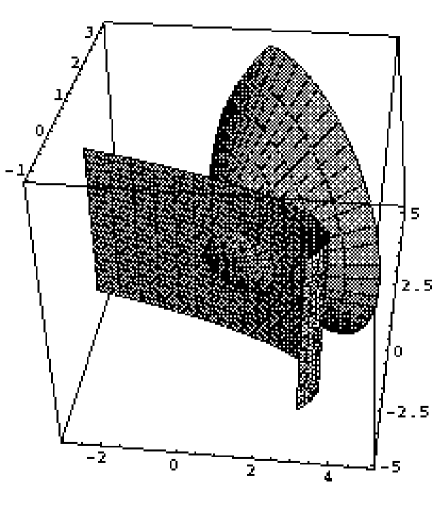
Figure 1: A typical intersection $M_{h,j}$ of the surfaces $P_{j}$ and $H_{j}^{-1}(h)$.

The Poisson bracket $\{\cdot,\cdot\}$ associated with the standard symplectic structure $\Omega$ on $\mathbb{R}^{4}$ defines a Poisson structure on the algebra of invariant polynomials with brackets

$$\{\Gamma_{1},\Gamma_{2}\}=\{\Gamma_{1},\Gamma_{3}\}=\{\Gamma_{1},\Gamma_{4}\}=0,$$ (5)

$$\{\Gamma_{2},\Gamma_{3}\}=\Gamma_{4},\quad\{\Gamma_{3},\Gamma_{4}\}=-2\Gamma_{3},\quad\{\Gamma_{4},\Gamma_{2}\}=-2\Gamma_{2}\,.$$ (6)

The momentum map of the $S^{1}$ action used for the reduction induces the Casimir $\Gamma_{1}$ in this Poisson bracket. In addition also the relation between the generators (3) given by $G$ is a Casimir. Accordingly the nonzero brackets give a Poisson structure on $\mathbb{R}^{3}$ with coordinates $(\Gamma_{2},\Gamma_{3},\Gamma_{4})$, that has the reduced spaces $P_{j}$ as its symplectic leaves. It can be written as

$$\{\Gamma_{2},\Gamma_{3}\}=\partial G/\partial\Gamma_{4},\quad\{\Gamma_{3},\Gamma_{4}\}=\partial G/\partial\Gamma_{2},\quad\{\Gamma_{4},\Gamma_{2}\}=\partial G/\partial\Gamma_{3}\,.$$ (7)

The reduced equations of motion are

$$\dot{\Gamma}_{2} =\{\Gamma_{2},H_{j}\}=\Gamma_{4}\frac{\partial H_{j}}{\partial\Gamma_{3}},$$ (8)

$$\dot{\Gamma}_{3} =\{\Gamma_{3},H_{j}\}=-\Gamma_{4},$$

$$\dot{\Gamma}_{4} =\{\Gamma_{4},H_{j}\}=-2\Gamma_{2}+2\Gamma_{3}\frac{\partial H_{j}}{\partial\Gamma_{3}}\,.$$

The integral curves of this flow are given by $M_{h,j}$, the intersection of $P_{j}$ and $H_{j}^{-1}(h)$. In general the intersection of these two manifolds is either empty or diffeomorphic to a circle. The preimage of any point in reduced phase space is the set of points in original phase space that are mapped to this point by the momentum map $J$. If one point in the preimage is known the others can be obtained by letting the flow of $J$ (i.e. the map $\Phi$) act on this point to get the complete fibre. This gives a circle unless starting in the origin. Therefore the preimage of a circle $M_{h,j}$ is a two dimensional torus $\mathbb{T}^{2}$ in the phase space of the original system.

Exceptions occur for equilibrium points of the reduced system. They occur either when the surface $H_{j}^{-1}(h)$ is tangent to $P_{j}$ or when $j=0$ and $H_{0}^{-1}(h)$ contains the singular point at the origin (which implies $h=0$). The preimage of the singular point is not a circle, because $\Gamma_{2}=\Gamma_{3}=0$ implies $q_{1}=q_{2}=p_{1}=p_{2}=0$ and this is a fixed point of the flow $\Phi$. This is the equilibrium point in the full system that undergoes the Hopf bifurcation. All other equilibrium points of the recuded system are reconstructed to periodic orbits of the full system; they are relative equilibria of $J$. The $S^{1}$ action generated by $J$ is not free. The origin is a fixed point, and this is the reason why singular reduction is needed in this example.

3 Energy-Momentum Map

Using the reduced system we can find the critical values of the energy momentum map

$$F:\mathbb{R}^{4}\to\mathbb{R}^{2},\qquad(p,q)\mapsto F(p,q)=(H(p,q),J(p,q))\,.$$ (9)

The values of the energy-momentum map are denoted by $(h,j)$. For every regular value of $F$ the preimage in phase space is a two dimensional torus. The critical values are determined from equilibrium points of the reduced system because their preimages are not $\mathbb{T}^{2}$. Since we are interested in a neighbourhood of the origin in phase space for small $\delta$ we will only consider a small neighbourhood of the origin in the image of the momentum map.

Consider the reduced equilibrium points caused by the singularity in the reduced space first. This singularity occurs for $j=0$. The singular point $(\Gamma_{2},\Gamma_{3},\Gamma_{4})=(0,0,0)$ has energy $h=0$. The equilibrium at the origin in phase space is therefore mapped to the origin in the image of the momentum map.

When $\delta>0$ the intersection $M_{0,0}$ restricted to a neighborhood of the origin in reduced phase space consists only of the origin. It reconstructs to an elliptic equilibrium. However, if $\delta<0$ then $M_{0,0}$ is a non-smooth circle with a corner, if it is compact. The preimage of $M_{0,0}$ is diffeomorphic to a pinched torus in this case.

Consider next the equilibrium points caused by a tangency of $P_{j}$ and $H_{j}^{-1}(h)$. At these critical values of $H_{j}$ the gradient of $H_{j}$ and the gradient of $G$ are parallel. Since $\partial G/\partial\Gamma_{4}=\Gamma_{4}$ the tangency may occur only on the hyperplane $\Gamma_{4}=0$. The intersections of $P_{j}$ and $H_{j}^{-1}(h)$ with this hyperplane are one branch of a hyperbola and a parabola, respectively. They are described by the equations

$$j^{2} =4\Gamma_{2}\Gamma_{3},$$ (10)

$$h =\omega j+Cj^{2}+\Gamma_{2}-\frac{(\delta+2Bj)^{2}}{8D}+2D\left(\Gamma_{3}+\frac{\delta+2Bj}{4D}\right)^{2}\,.$$ (11)

At the extremal values of $h$ the two curves are tangent. Eliminating $\Gamma_{2}$ in (10) using (11) gives a polynomial of degree 3 in $\Gamma_{3}$ depending on $j$ and $h$

$$Q_{3}(\Gamma_{3}):=-8D\Gamma_{3}^{3}-4(\delta+2Bj)\Gamma_{3}^{2}+4(h-\omega j-Cj^{2})\Gamma_{3}-j^{2}=0\,.$$ (12)

This polynomial $Q_{3}(\Gamma_{3})$ gives the value of $\Gamma_{4}^{2}$ obtained from $G=0$ and expressed in terms of $\Gamma_{3}$. The tangency between the hyperbola (10) and the parabola (11) occurs when $Q_{3}$ has a double root. We will first discuss all values of $(h,j)$ for which a tangency occurs, irrespective of them satisfying the constraints $\Gamma_{2}\geq 0$ and $\Gamma_{3}\geq 0$. In a second step the critical values of the energy momentum will be found by consideration of these constraints.

Figure 2: The discriminant surface of the polynomial $Q_{3}$. The critical values of the energy-momentum map are contained in the discriminant surface. The small triangular part for $\delta>0$ is not in the image of the energy-momentum map for $D<0$. The figures correspond to the cases of $\delta=-0.15$ and $\delta=0.15$ respectively. ($B=C=-D=\omega=1.0$)

To parametrize all tangencies we make the ansatz $Q_{3}(z)=-8D(z-d/2)^{2}(z+s^{2}/D/2)$ with parameters $d$ and $s$ parametrising the double and single root of $Q_{3}$, respectively. This leads to the parametrisation of the tangencies by $s\in\mathbb{R}$

$$j_{\text{crit}}(s) =sd(s),\qquad d(s)=\frac{\delta-s^{2}}{2(Bs-D)},\quad$$ (13)

$$h_{\text{crit}}(s) =\omega j_{\text{crit}}(s)+Cj_{\text{crit}}(s)^{2}-2d(s)^{2}D+2sj_{\text{crit}}(s)\,.$$

The root $\Gamma_{3}=-s^{2}/D/2$ always has the opposite sign than $D$. The curve $(h_{\text{crit}}(s),j_{\text{crit}}(s))$ has singular points when $s$ has one of the singular values satisfying $2Bs^{3}-3s^{2}D+\delta D=0$. The number of singular points changes when the discriminant $108\delta D^{2}(D^{2}-\delta B^{2})$ vanishes. For small $|\delta|$ the only change occurs at $\delta=0$, see Fig. 2, for two slices of the “swallowtail”.

For $\delta>0$ the curve has two singular points near the origin for some $s\in(-\sqrt{\delta},\sqrt{\delta})$. The two singular points are located at

$$h^{*} =\pm\frac{\omega}{\sqrt{27}D}\delta^{3/2}+\frac{2B\omega-3D}{18D^{2}}\delta^{2}\pm O(\delta^{5/2})$$ (14)

$$j^{*} =\pm\frac{1}{\sqrt{27}D}\delta^{3/2}+\frac{B}{9D^{2}}\delta^{2}\pm O(\delta^{5/2})$$

for small $\delta\geq 0$. The curve of critical values has a self-intersection at $s^{2}=\delta$. The intersection point at the origin marks the elliptic equilibrium with eigenvalues $i(\omega\pm\sqrt{\delta})$. The slopes of the intersecting curves are given by the imaginary parts of the eigenvalues.

For $\delta<0$ the equilibrium point at the origin is unstable with eigenvalues $\sqrt{-\delta}+i\omega$. The curve $(h_{\text{crit}}(s),j_{\text{crit}}(s))$ does not intersect the origin, instead the origin is now an isolated critical point. The curve is above the origin for $D>0$ and below for $D<0$, e.g. the point with $s=0$ is at $(h,j)=(-\delta^{2}/8/D,0)$.

Only tangencies that occur with the part of the hyperbola in the positive quadrant give critical values of the energy-momentum map since $\Gamma_{2}$ and $\Gamma_{3}$ are both non-negative. The double roots $d(s)$ near $s=0$ occurs at

$$d(s)=-\frac{\delta}{2D}-O(s)\,.$$ (15)

Near the intersection at the origin around $s=\pm\delta$ the double root is

$$d(s)=\frac{\sqrt{\delta}}{D}(\pm s-\sqrt{\delta})+O((\pm s-\sqrt{\delta})^{2})$$ (16)

If $D>0$ this implies that the smooth curve for $\delta<0$ is in the (boundary of the) image of the energy-momentum map, while the part of the curve with $s\in(-\sqrt{\delta},\sqrt{\delta})$ is not in the image for $\delta>0$. Conversely for $D<0$ the smooth curve for $\delta<0$ is not in the image, while for $\delta>0$ only the triangular part with $s\in[-\sqrt{\delta},\sqrt{\delta}]$ is in the image. Therefore the union of the bifurcation diagram (i.e. the set of critical values of the energy-momentum map) for $+D$ and $-D$ gives the discrimiant of the polynomial $Q_{3}$.

The type of the preimage of the critical values is determined by the character of the intersection $M_{h,j}$. The positive half of the hyperboloid $G$ projects onto the area above the hyperbola given by $j^{2}\leq 4\Gamma_{2}\Gamma_{3}$. If the parabola (11) touches the boundary of the area from the outside, the preimage in the full phase space is a circle, hence a stable periodic orbit. If the parabola touches from the inside, the preimage is a circle with a separatrix, hence an unstable periodic orbit. This can only occur when $D<0$, because then the parabola is open upwards. It only occurs when $\delta>0$ for $s$ between the two singular values enclosing zero. In all other cases the parabola touches from the outside. The complete bifurcation scenario in the two cases therefore is as follows, see Figure 2 for illustration.

The case $D>0$: For $\delta<0$ there is an isolated focus-focus point at the origin and a smooth curve of elliptic periodic orbits nearby. For $\delta>0$ there is an elliptic equilibirum point and there are two families of elliptic periodic orbits (non-linear normal modes) emanating from the equilibrium.

The case $D<0$: For $\delta<0$ there is nothing but an isolated focus-focus point. For $\delta>0$ there is an elliptic equilibirum point and there are two families of elliptic periodic orbits (non-linear normal modes) emanating from the equilibrium. Both families terminate in a cusp formed with the same family of hyperbolic periodic orbits. The set of critical values therefore forms a triangle with two cuspoidal corners and one regular corner at the origin.

4 Actions

From now on we shall assume the parameter $D$ to be a positive number. In this case each constant energy level is compact and by the Liouville-Arnold theorem it is possible to define action-angle coordinates near regular points of $F$. To construct the second action we need to integrate a 1-form $\Theta$ over $M_{J,h}$, where the differential ${\rm d}\Theta$ coincide with a symplectic structure induced by the quotient map $\pi_{h,j}:\mathbb{R}^{4}\to F^{-1}(h,j)/S^{1}$ from the original phase space, i.e. ${\rm d}\Theta=(\pi_{h,j}^{-1})^{\*}\Omega|_{TM_{h,j}}$. To find the form $\Theta$ we chose $\Gamma_{3}$ as one variable and find its conjugate variable by solving the equation

$$\{f(\Gamma_{2},\Gamma_{3},\Gamma_{4}),\Gamma_{3}\}=1.$$ (17)

A solution of (17) is the function

$$f(\Gamma_{2},\Gamma_{3},\Gamma_{4})=\frac{\Gamma_{4}}{2\Gamma_{3}}.$$ (18)

Then the canonical one form is $\Theta=\frac{\Gamma_{4}}{2\Gamma_{3}}{\rm d}\Gamma_{3}$ and we obtain

$$J_{2}(h,j)=\frac{1}{2\pi}\oint\limits_{M_{h,j}}\frac{\Gamma_{4}{\rm d}\Gamma_{3}}{2\Gamma_{3}}=\frac{1}{2\pi}\oint\limits_{M_{h,j}}\frac{\sqrt{4\Gamma_{2}\Gamma_{3}-j^{2}}}{2\Gamma_{3}}\mathrm{d}\Gamma_{3}$$ (19)

for the second action. Here $\Gamma_{4}$ is considered as a function of $\Gamma_{3}$ by first expressing $\Gamma_{4}$ in terms of $\Gamma_{2}$ and $\Gamma_{3}$ on the reduced phase space $P_{j}$ and then by expressing $\Gamma_{2}$ in terms of $\Gamma_{3}$ using $H_{j}=h$. As a result the polynomial $Q_{3}$ is found as already given by (12). The action integral hence is defined on the elliptic curve

$${\cal E}=\{(w,z):w^{2}=Q_{3}(z)\}\,.$$ (20)

Recall that $w=\Gamma_{4}$ on $P_{j}$. Now the action integral can be written as

$$J_{2}=\frac{1}{4\pi}\oint\frac{w}{z}\mathrm{d}z\,.$$ (21)

It is an integral of the third kind with a pole at $z=0$ and residue $\pm\mathrm{i}j/4\pi$.

The formula for the action can also be obtained in a classical way, using polar coordinates as in [18]. A slightly different coordinate transformation illucidates the connection between the two approaches. The new symplectic structure is $\Omega=\mathrm{d}P_{g}\wedge\mathrm{d}g+\mathrm{d}J\wedge\mathrm{d}\phi$ and “symplectic polar coordinates” valid for $q_{1}^{2}+q_{2}^{2}>0$ are introduced by

$$q_{1}=\sqrt{2g}\cos\varphi,\quad p_{1}=P_{g}\sqrt{2g}\cos\varphi-J\frac{\sin\varphi}{\sqrt{2g}},$$ (22)

$$q_{2}=\sqrt{2g}\sin\varphi,\quad p_{2}=P_{g}\sqrt{2g}\sin\varphi+J\frac{\cos\varphi}{\sqrt{2g}}.$$ (23)

The invariant polynomials are related to these coordinates by

$$\Gamma_{1}=J,\quad\Gamma_{2}=gP_{g}^{2}+\frac{J^{2}}{4g},\quad\Gamma_{3}=g,\quad\Gamma_{4}=2gP_{g}\,.$$ (24)

In these variables the Hamiltonian takes the form

$$H=gP_{g}^{2}+\frac{J^{2}}{4g}+\omega J+(\delta+2BJ)g+CJ^{2}+2Dg^{2}\,,$$ (25)

and the equations of motion are

$$\dot{\varphi} =\frac{J}{2g}+\omega+2Bg+2CJ\,,$$ (26)

$$\dot{g} =2gP_{g}\,,$$

$$\dot{P}_{g} =P_{g}^{2}-\frac{J^{2}}{4g^{2}}+(\delta+2BJ)+4Dg\,.$$

Solving the Hamiltonian (25) for $P_{g}^{2}$ gives

$$P_{g}^{2}=\frac{Q_{3}(g)}{4g^{2}}$$ (27)

so that the action integral (19) is obtained from integrating the canonical form $P_{g}\mathrm{d}g$ over a path with constant $\phi$.

5 Rotation Number

We want to check the isoenergetic non-degeneracy condition of the KAM theorem. A torus is non-degenerate in this sense if the map from the actions restricted to a constant energy surface $H=h$ to the frequency ratios $\omega_{1}:\omega_{2}$ is non-degenerate. This means that the frequency ratio (or rotation number) $W=\omega_{1}/\omega_{2}$ changes when the torus is changed at constant energy. On a local transversal Poincaré section this condition is called twist condition.

In our case this is equivalent to the non-vanishing of the partial derivative of the rotation number $W$ with respect to the action $J_{1}$. By definition the winding number is the ratio of frequences $\omega_{1},\omega_{2}$, corresponding to the actions $J_{1}$ and $J_{2}$. If the Hamiltonian is expressed in terms of $J=J_{1}$ and $J_{2}$ then $\partial_{1}H(J_{1},J_{2})=\omega_{1}$ and $\partial_{2}H(J_{1},J_{2})=\omega_{2}$. Therefore we find by implicit differentiation of $J_{2}(h,j)=j_{2}$ that

$$W=\frac{\omega_{1}}{\omega_{2}}=-\frac{\partial J_{2}}{\partial j}.$$ (28)

However, the simplest way to obtain $W$ is to observe that it is the advance of the angle $\phi$ conjugate to $J$ during the time of a full period of the motion of $g=\Gamma_{3}$. The period of the motion is obtained from the reduced equation of motion $\dot{\Gamma}_{3}=-\Gamma_{4}$. On $P_{j}$ this gives

$$\dot{\Gamma}_{3}^{2}=4\Gamma_{2}\Gamma_{3}-j^{2}$$ (29)

and eliminating $\Gamma_{2}$ by using $H_{j}=h$ gives

$$\left(\frac{\mathrm{d}\Gamma_{3}}{\mathrm{d}t}\right)^{2}=4\Gamma_{3}\Gamma_{2}(\Gamma_{3};h,j)-j^{2}\,.$$ (30)

By separation of variables we obtain the period of the reduced motion as

$$T(h,j)=\oint\frac{\mathrm{d}\Gamma_{3}}{\sqrt{4\Gamma_{3}\Gamma_{2}-j^{2}}}=\oint\frac{\mathrm{d}z}{w}\,.$$ (31)

To obtain the advance of $\phi$ in time $T$ we change the time $t$ in (26) to “time” $\Gamma_{3}$ and find

$$\frac{\mathrm{d}\phi}{\mathrm{d}\Gamma_{3}}=\frac{j+2\Gamma_{3}(\omega+2Cj)+B(2\Gamma_{3})^{2}}{2\Gamma_{3}\Gamma_{4}}$$ (32)

Expressing $\Gamma_{4}$ in terms of $\Gamma_{3}$ on the reduced phase space $P_{j}$ as before the period of the solution of this equation gives the rotation number $2\pi W$. The rotation number $W$ can therefore be written as a linear combination of integrals of the first, second and third kind,

$$2\pi W(h,j)=(\omega+2Cj)\oint\frac{\mathrm{d}z}{w}+2B\oint\frac{z\,\mathrm{d}z}{w}+\frac{j}{2}\oint\frac{\mathrm{d}z}{zw}\,.$$ (33)

The first integral is of the first kind and proportional to the period $T$. The last integral is of the third kind and propotional to the action $J_{2}$. When $D>0$ the polynomial $Q_{3}$ has three real roots, which we denote by $z_{\text{neg}},z_{\text{min}},z_{\text{max}}$, such that $z_{\text{neg}}\leq 0\leq z_{\text{min}}\leq z_{\text{max}}$. The closed loop integrals encircle the finite range of positive $Q_{3}$, and therefore can be rewritten by the rule

$$\oint=2\int\limits_{z_{\text{min}}}^{z_{\text{max}}}\,.$$ (34)

The elliptic integrals can be transformed to Legendre standard integrals $K(k)$, $E(k)$, and $\Pi(k)$ of the first, second, and third kind, respectively, with modulus $k$ and characteristic (or parameter) $n$ given by

$$k^{2}=\frac{z_{\text{max}}-z_{\text{min}}}{z_{\text{max}}-z_{\text{neg}}},\quad n=\frac{z_{\text{max}}-z_{\text{min}}}{z_{\text{max}}}\,.$$ (35)

The result is

$$W(j,h)=\frac{(2Bz_{\text{neg}}+\omega+2Cj)K(k)+2B(z_{\text{max}}-z_{\text{neg}})E(k)+j\Pi(n,k)/({2z_{\text{max}}})}{\pi\sqrt{2D}\sqrt{z_{\text{max}}-z_{\text{neg}}}}.$$ (36)

Explicit formulas for the vanishing of the twist $\partial W/\partial j$ can be derived from this.

The rotation number is a complicated function of the constants of motion $(h,j)$. The level lines of this function are shown in Fig. 3 and 4. Near the cases where the discriminant of the elliptic curve $E$ defined by $Q_{3}$ in (20) vanishes, simpler formulas can be derived. This occurs either at the boundary of the image of the energy-momentum map described by (13), or at the isolated focus-focus point $(h,j)=(0,0)$ inside the image. In the next section we will treat the latter case.

6 Rotation Number near the Focus-Focus Point

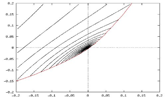
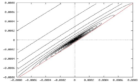
Figure 3: The level lines of the rotation number on the $(j,h)$ plane. The bifurcation parameter $\delta$ is decreasing from top to bottom, $\delta=-0.2,-0.15,-0.02$ ($\omega=B=C=-D=1$). The level lines are spirals. The boundary of the image of the energy momentum map given by a family of relative equilibria is also shown.

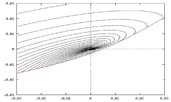
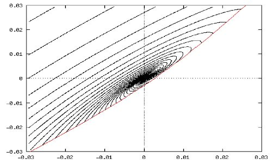
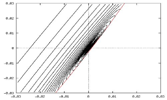
Figure 4: The level lines of the rotation number on the $(j,h)$ plane. Here the imaginary part of the eigenvalue $\omega$ is changed, from top to bottom $\omega=1/2,1,2$ ($\delta=-0.15,B=C=-D=1$).

We introduce a small parameter by scaling $h$ and $j$ by epsilon, hence replace $h\to h\varepsilon$, $j\to j\varepsilon$. This means that we obtain an expansion that approaches the origin on a ray. Alternatively one can view $\varepsilon$ as a formal expansion parameter that keeps track of the fact that both, $h$ and $j$ are small and of the same order. The focus point only exists for $\delta<0$, which we henceforth assume. At the origin $Q_{3}$ reduces to

$$Q_{3}(z;h=0,j=0)=-4z^{2}(2Dz+\delta)\,,$$ (37)

so that $z_{\text{min}}$ and $z_{\text{neg}}$ collide at 0 and $z_{\text{max}}=-\delta/2/D$. The roots can be expanded in power series in $\varepsilon$, and the result is

$$2z_{\text{neg}} =-\frac{l+\rho}{\alpha}\varepsilon+O(\varepsilon^{2}),$$ (38)

$$2z_{\text{min}} =-\frac{l-\rho}{\alpha}\varepsilon+O(\varepsilon^{2}),$$

$$2z_{\text{max}} =\frac{\alpha^{2}}{D}+2\frac{Dl-jB\alpha}{D\alpha}\varepsilon+O(\varepsilon^{2})\,.$$

Here and in the following we use the abbreviations

$$l=\frac{h-\omega j}{\alpha},\quad\rho^{2}=l^{2}+j^{2},\quad f=\frac{D}{\alpha^{3}},\quad\alpha=\sqrt{-\delta}\,.$$ (39)

The expressions are only real in the case $\delta<0$, otherwise the focus-focus point does not exist. Inserting this into (35) gives

$$k^{2} =1-2f\rho\varepsilon+O(\varepsilon^{2}),$$ (40)

$$n =1+f(l-\rho)\varepsilon+O(\varepsilon^{2}).$$

For small $\varepsilon$ both, $k$ and $n$ are close to 1 and they satisfy the inequality

$$k^{2}\leq n\leq 1\,.$$ (41)

In the limit $k\to 1$ the elliptic integrals are singular, but there are expansions that include the logarithmically diverging terms. The details of this expansion can be found in the appendix. The result for the rotation number is

$$2\pi W(h,j)=-\frac{\omega}{\alpha}\ln\rho-\tan^{-1}\frac{j}{l}+O(1)\,.$$ (42)

Keeping terms only up to order 1 is enough because when the twist condition $\partial W/\partial j$ is calculated the present terms both give singular contributions, the constant term disappears and the first order term in $\varepsilon$ is very small compared to the singular terms. Note that $W$ is not a single valued function. The fact that $\tan^{-1}(j/l)/2\pi$ changes by one when the origin is encircled is an expression of the monodromy of this focus-focus point, see [7]. The expression given by the elliptic integrals, see the appendix, gives a continuous function which is, however, not differentiable when $j=0$.

The level lines of $W$ are spirals, which are easily parametrized in polar coordinates with the radius $\rho$ as parameter. Instead of viewing these spirals as the level lines of $W$ where $W$ is a many-valued function, it might be easier to see them as the integral curves of a flow in the plane that has an equilibrium point at $h=j=0$. The linear approximation to this flow is best written in complex notation $z=l+\mathrm{i}j$ so that $\dot{z}=\lambda z$ where $\lambda=\alpha+\mathrm{i}\omega$. Therefore we may formulate the result like this: The level lines of $W$ are the integral curves of a planar node with the same eigenvalue as the focus-focus point.

Calculating the leading order condition for the vanishing of twist is easily done by differentiating the first two terms of the expansion with respect to $j$. The result is that

$$\frac{\partial W}{\partial j}=0\quad\Rightarrow\quad h(\omega^{2}-\alpha^{2})=j\omega(\omega^{2}+\alpha^{2})\,.$$ (43)

This means that the twist vanishes on a line that has a tangent whose slope at the focus point can be read of from the above expression as

$$\frac{h}{j}=\omega\frac{\omega^{2}+\alpha^{2}}{\omega^{2}-\alpha^{2}}\,.$$ (44)

In particular this slope only depends on the eigenvalue of the focus-focus point. Approaching the bifurcation point $\alpha\to 0$, and hence the slope approaches $\omega$, see Fig. 3 and 4.

7 Vanishing Twist of Periodic Orbits

Now we consider the vanishing of the twist for the relative equilibria $(h_{\text{crit}}(s),j_{\text{crit}}(s))$ in the boundary of the image of the energy-momentum map. First we rescale the parameters, in order to keep the formulas manageable:

$$B=\frac{Db}{\omega},\ \ C=\frac{Dc}{\omega^{2}},\ \ \mu=\frac{\delta}{\omega^{2}},\ \ j=\frac{\hat{j}\omega^{3}}{D},\ \ h=\frac{\hat{h}\omega^{4}}{D},\ \ z=\frac{\zeta\omega^{2}}{D}.$$ (45)

Note that when $\delta<0$, which is the case we are interested here, we have $\mu=-\alpha^{2}/\omega^{2}$. In terms of the new parameters the polynomial $Q(z)$ becomes

$$Q(z)=\frac{\omega^{6}}{D^{3}}\hat{Q}(\zeta),\ \ \hat{Q}(\zeta)=-(\zeta^{3}+(\mu+2b\hat{j})\zeta^{2}+2(\hat{j}+c\hat{j}^{2}-\hat{h})\zeta+\hat{j}^{2}),$$ (46)

and the derivative $\partial W/\partial j$ is

$$\frac{\partial W}{\partial j}(j,h)=\frac{D}{4\pi\omega^{3}}\left(\oint\frac{(1+2c\zeta){\rm d}\zeta}{\zeta\hat{Q}^{1/2}(\zeta)}+\oint\frac{(b\zeta^{2}+(1+2c\hat{j})\zeta+\hat{j})^{2}{\rm d}\zeta}{\zeta\hat{Q}^{3/2}(\zeta)}\right).$$ (47)

The parametrisation of the critical values has already been obtained in (13). After the scaling it reads

$$\hat{d}(s)=\frac{\mu-s^{2}}{2(bs+1)},\quad\hat{j}_{\text{crit}}(s)=s\hat{d}(s),\quad\hat{h}_{\text{crit}}=\omega\hat{j}_{\text{crit}}(s)+c\hat{j}^{2}_{\text{crit}}(s)+2\hat{d}(s)^{2}+2s\hat{j}_{\text{crit}}(s)\,.$$ (48)

On the curve $(\hat{j}_{\text{crit}}(s),\hat{h}_{\text{crit}}(s))$ the integrals on the right hand side of (47) can be computed by the method of residues. Replacing $\hat{j}$ and $\hat{h}$ wherever they appear by their critical values parametrised by $s$ gives a condition for the vanishing of the twist on the curve of critical values. It implies the following polynomial equation

$$R_{9}(s)=\sum\limits_{k=0}^{9}a_{k}s^{k}=0,$$ (49)

where

$$a_{0}= -12\mu-4(4+b)\mu^{2}-(3b^{2}-16c)\mu^{3},$$ (50)

$$a_{1}= -24(5+b)\mu-4(b+b^{2}-6c)\mu^{2}+4bc\mu^{3},$$

$$a_{2}= -84-12(1+14b+b^{2})\mu+3(15b^{2}-8c+8bc)\mu^{2}-12c^{2}\mu^{2},$$

$$a_{3}= 4(30-66b)+16(b+b^{2}+9c)\mu+(24b^{3}-52bc)\mu^{2},$$

$$a_{4}= 12(5+25b-23b^{2})+(64b^{3}-29b^{2}+192c+336bc)\mu-4c(16b^{2}+15c)\mu^{2},$$

$$a_{5}= -12(8b^{3}-31b^{2}-7b+14c)-12b(12b^{2}-29c-16bc)\mu-96bc^{2}\mu^{2},$$

$$a_{6}= 320b^{3}+83b^{2}-312c-360bc-(96b^{4}-64b^{2}c-156c^{2})\mu,$$

$$a_{7}= 4b(32b^{3}+38b^{2}-171c-48bc)-64bc(2b^{2}-3c)\mu,$$

$$a_{8}= 12(8b^{4}-32b^{2}c-7c^{2}),$$

$$a_{9}= -96bc^{2}.$$

The first two coefficients $a_{0}$ and $a_{1}$ are of the first order in $\mu$, while $a_{2}$ is non-zero for small $\mu$. Therefore the roots of $R_{9}$ can be expanded in powers of $|\mu|^{1/2}=\alpha/\omega$, and for small $|\mu|$ there are only two roots in a $|\mu|^{1/2}$ neighborhood of the origin. The result is

$$s_{\pm}=\pm\sqrt{\frac{-\mu}{7}}+\frac{4}{7}(10-b)\mu+O(|\mu|^{3/2}).$$ (51)

The critical values of the twistless periodic orbit are then given by

$$\hat{j}_{\pm} =\pm\frac{4}{7}\sqrt{\frac{-\mu^{3}}{7}}+\frac{8}{7^{3}}(25-6b)\mu^{2}+O(|\delta|^{5/2}),$$ (52)

$$\hat{h}_{\pm} =\pm\frac{4}{7}\sqrt{\frac{-\mu^{3}}{7}}+\frac{8}{7^{3}}(43/2-6b)\mu^{2}+O(|\delta|^{5/2})\,.$$ (53)

This gives two points in each of the Figures 3 and 4, at which the curve of vanishing twist emanating from the origin crosses the boundary of the image of the energy-momentum map. The value of the rotation number at these points is

$$\sqrt{5}W_{\pm}=\frac{1}{2}\sqrt{\frac{7}{-\mu}}\pm\frac{1}{7}(5-2b)+O(|\mu|^{1/2})\,.$$ (54)

We have now treated both limiting cases, that near the focus-focus point, and that near the elliptic relative equilibria. The curve of vanishing twist for all values in between can in principle be computed from the derivative of (36), and will connect the results from the two limiting cases for small values of $\delta$.

Appendix A Expansion of $W$

We need to expand the Legendre standard integrals $K$, $E$, and $\Pi$ in the limit $k\to 1$. For the expansion of the integral of the third kind it is important to take the inequality $k^{2}\leq n\leq 1$ (41) into account. In this limit the following formulas can e.g. be found in [1]:

$$\Pi(n,k)=K(k)+\frac{1}{2}\pi{\cal R}(1-\Lambda_{0}(\theta,k)),$$ (55)

$${\cal R}=\left(\frac{n}{(1-n)(n-k^{2})}\right)^{1/2}=\left(\frac{(z_{\text{neg}}-z_{\text{max}})z_{\text{max}}}{z_{\text{neg}}z_{\text{min}}}\right)^{1/2}\,.$$ (56)

Here $\Lambda_{0}$ is Heumann’s Lambda function, which can be expressed in terms of incomplete elliptic integrals $F(\theta,k)$ and $E(\theta,k)$ of the first and the second kind, respectively, as

$$\Lambda_{0}(\theta,k)=\frac{2}{\pi}\left(K(k)E(\theta,k^{\prime})-(K(k)-E(k))F(\theta,k^{\prime})\right),$$ (57)

$$\theta=\arcsin\sqrt{\frac{1-n}{1-k^{2}}}=\arcsin\sqrt{\frac{z_{\text{min}}(z_{\text{max}}-z_{\text{neg}})}{z_{\text{max}}(z_{\text{min}}-z_{\text{neg}})}}\,.$$ (58)

Note that the complementary modulus $k^{\prime}=\sqrt{1-k^{2}}$ and the parameter satisfy

$$k^{\prime 2}=1-k^{2}=O(\varepsilon),\quad 1-n=O(\varepsilon)\,,$$

see (40). Accordingly $k^{\prime 2}$ and $1-n$ are of order $\varepsilon$, while $\theta$ is not small but of order 1. The prefactor $\cal R$ in (55) cancels with the prefactor of $\Pi$ in (36), up to a factor of $1/2$. Therefore we find the (still exact) formula

$$W=c_{1}K+c_{2}E+\frac{1}{2}(1-\Lambda_{0}(\theta,k))$$ (59)

where with $\sqrt{z_{\text{max}}-z_{\text{neg}}}=\alpha/\sqrt{2D}+O(\varepsilon)$ it follows

$$\pi c_{1} =\frac{\omega+2Bz_{\text{neg}}+2Cj+j/(2z_{\text{max}})}{\sqrt{2D}\sqrt{z_{\text{max}}-z_{\text{neg}}}}=\frac{\omega}{\alpha}+O(\varepsilon),$$ (60)

$$\pi c_{2} =\frac{2B\sqrt{z_{\text{max}}-z_{\text{neg}}}}{\sqrt{2D}}=\frac{B\alpha}{D}+O(\varepsilon)\,.$$ (61)

The elliptic integrals in the limit $k^{\prime}\to 0$ have a logarithmic divergence of leading order

$$\Lambda=\log\frac{4}{k^{\prime}}\,.$$ (62)

The convergent expansions in this limit are

$$K(k)=\Lambda+\frac{\Lambda-1}{4}k^{\prime 2}+O(\Lambda k^{\prime 4}),$$ (63)

$$E(k)=1+\frac{1}{2}\left(\Lambda-\frac{1}{2}\right)k^{\prime 2}+O(\Lambda k^{\prime 4}),$$ (64)

The incomplete elliptic integrals of modulus $k^{\prime}$ have regular expansions since $k^{\prime}\to 0$, so that

$$F(\theta,k^{\prime})-E(\theta,k^{\prime})=\int\limits_{0}^{\theta}\frac{k^{\prime 2}\sin^{2}\varphi{\rm d}\varphi}{\sqrt{1-k^{\prime 2}\sin^{2}\varphi}}=\left(\frac{\theta}{2}-\frac{\sin 2\theta}{4}\right)k^{\prime 2}+O(k^{\prime 4}),$$ (65)

$$F(\theta,k^{\prime})=\int\limits_{0}^{\theta}\frac{{\rm d}\varphi}{\sqrt{1-k^{\prime 2}\sin^{2}\varphi}}=\theta+\frac{1}{2}\left(\frac{\theta}{2}-\frac{\sin 2\theta}{4}\right)k^{\prime 2}+O(k^{\prime 4})\,.$$ (66)

For the Heumann Lambda function this gives

$$\Lambda_{0}(\theta,k)=\frac{2}{\pi}\left(\theta+\frac{1}{4}\left(\Lambda-\frac{1}{2}\right)\sin(2\theta)k^{\prime 2}+O(\Lambda k^{\prime 4})\right).$$ (67)

The leading order terms in the expansion of (36) come from the diverging $K$. Since $E\to 1$ for $k\to 1$ there is only a constant contribution from $c_{2}$. From $\Lambda_{0}$ the leading term is merely $\theta$, so that all together

$$\pi W=\frac{\omega}{\alpha}\Lambda+\frac{\pi}{2}-\theta+\frac{B\alpha}{D}+O(\varepsilon)$$ (68)

It remains to understand the parameter dependence of $\theta$. Expanding $\theta$ gives

$$2\theta\approx 2\arcsin\sqrt{\frac{\rho-l}{2\rho}}+O(\varepsilon).$$ (69)

This can be simplified using the relation

$$2\arcsin{\beta}=\arctan{\gamma}\quad\Rightarrow\quad\gamma=2\frac{\sqrt{1-\beta^{2}}\beta}{1-2\beta^{2}}\,.$$ (70)

Inserting $\beta^{2}=(\rho-l)/(2\rho)$ and using $\rho^{2}=l^{2}+j^{2}$ gives $\gamma=j/l$, so that (42) is proved. Note that when $j=0$ we have $\rho=l$ and the root $z_{\text{min}}$ collides with the pole at $z=0$ in the third kind integral. This is the place where the dependence on the parameters of $\Pi(n,k)$ is continuous, but not smooth.

References

- [1] Milton Abramowitz and Irene A. Stegun, editors. Handbook of mathematical functions with formulas, graphs, and mathematical tables. Dover Publications Inc., New York, 1992. Reprint of the 1972 edition.
- [2] V. I. Arnold, V. V. Kozlov, and A. I. Neishtadt. Mathematical aspects of classical and celestial mechanics. Springer-Verlag, Berlin, 1997. Translated from the 1985 Russian original by A. Iacob, Reprint of the original English edition from the series Encyclopaedia of Mathematical Sciences [Dynamical systems. III, Encyclopaedia Math. Sci., 3, Springer, Berlin, 1993; MR 95d:58043a].
- [3] Richard H. Cushman and Larry M. Bates. Global aspects of classical integrable systems. Birkhäuser Verlag, Basel, 1997.
- [4] D. del Castillo-Negrette, J.M. Greene, and P.J. Morrison. Area preserving nontwist maps: Periodic orbits and transition to chaos. Physica D, 91(1):1–23, 1996.
- [5] A. Delshams and R. de la Llave. KAM theory and a partial justification of Greene’s criterion for nontwist maps. SIAM J. Math. Anal., 31(6):1235–1269 (electronic), 2000.
- [6] J. J. Duistermaat. Bifurcation of periodic solutions near equilibrium points of Hamiltonian systems. In Bifurcation theory and applications (Montecatini, 1983), volume 1057 of Lecture Notes in Math., pages 57–105. Springer, Berlin, 1984.
- [7] J. J. Duistermaat. The monodromy in the Hamiltonian Hopf bifurcation. Z. Angew. Math. Phys., 49(1):156–161, 1998.
- [8] H. R. Dullin and A. V. Ivanov. (Vanishing) twist in the saddle-centre and period-doubling bifurcation. (preprint http://arxiv.org/abs/nlin.CD/0305033), 2003.
- [9] H. R. Dullin and J. D. Meiss. Twist singularities for symplectic maps. Chaos, 13(1):1–16, 2003.
- [10] H. R. Dullin, J. D. Meiss, and D. G. Sterling. Generic twistless bifurcations. Nonlinearity, 13:203–224, 2000.
- [11] J. E. Howard and J. Humpherys. Nonmonotonic twist maps. Physica D, 80(3):256–276, 1995.
- [12] J.E. Howard and S.M. Hohs. Stochasticity and reconnection in hamiltonian systems. Physical Review A, 29:418, 1984.
- [13] R. Moeckel. Generic bifurcations of the twist coefficient. Ergodic Theory Dynam. Systems, 10(1):185–195, 1990.
- [14] J. A. Montaldi, R. M. Roberts, and I. N. Stewart. Periodic solutions near equilibria of symmetric Hamiltonian systems. Philos. Trans. Roy. Soc. London Ser. A, 325(1584):237–293, 1988.
- [15] J. Moser. Periodic orbits near an equilibrium and a theorem by Alan Weinstein. Comm. Pure Appl. Math., 29(6):724–747, 1976.
- [16] Helmut Rüssmann. Nondegeneracy in the perturbation theory of integrable dynamical systems. In Number theory and dynamical systems (York, 1987), volume 134 of London Math. Soc. Lecture Note Ser., pages 5–18. Cambridge Univ. Press, Cambridge, 1989.
- [17] C. Simó. Invariant curves of analytic perturbed nontwist area preserving maps. Regular & Chaotic Dynamics, 3:180–195, 1998.
- [18] A. G. Sokol′skiĭ. On stability of an autonomous Hamiltonian system with two degrees of freedom under first-order resonance. Prikl. Mat. Meh., 41(1):24–33, 1977.
- [19] Jan-Cees van der Meer. The Hamiltonian Hopf bifurcation, volume 1160 of Lecture Notes in Mathematics. Springer-Verlag, Berlin, 1985.
- [20] Alan Weinstein. Normal modes for nonlinear Hamiltonian systems. Invent. Math., 20:47–57, 1973.