Fluctuations of energy injection rate in a shear flow

Abstract

We study the instantaneous and local energy injection in a turbulent shear flow driven by volume forces. The energy injection can be both positive and negative. Extremal events are related to coherent streaks. The probability distribution is asymmetric, deviates slightly from a Gaussian shape and depends on the position in shear direction. The probabilities for positive and negative injection are exponentially related, but the prefactor in the exponent varies across the shear layer.

1 Introduction

Turbulent flows are a characteristic example for a dissipative macroscopic system that is driven steadily far from equilibrium. Energy of motion is dissipated continuously due to friction between the fluid parcels and has to be fed in by some kind of stirring or a large scale shear gradient in order to sustain the turbulent state [1]. Although this picture is as old as turbulence research itself, not much is known about the interplay between the rates of energy dissipation and energy input. Several recent experimental efforts have focussed on studies of the energy input rate into turbulent systems: Ciliberto and Laroche [2] extracted the buoyant energy input in turbulent Rayleigh-Bénard convection, Goldburg et al. [3] measured the power transfered to a liquid crystal in a chaotic regime above the electrohydrodynamic instability, Pinton et al. and Cadot et al. studied the injection rate statistics with von Karman swirling flow experiments [4, 5, 6, 7].

On the level of a macroscopic description energy dissipation in a turbulent flow is always positive, reflecting the irreversibiliy of the dynamics through a direct relation between dissipation and entropy production. While in the mean energy dissipation and energy uptake are equal, the fluctuations of energy uptake are much less constraint and can take both signs.

Fluctuations of the energy dissipation have recently attracted attention in connection with the observation that in the case of reversible non-equilibrium systems both signs for the entropy production are possible, but that the entropy reduction is exponentially suppressed compared to entropy production [8, 9] (for a comprehensive review see [10]). For hydrodynamic systems these ideas do not strictly apply, since the Navier-Stokes equation is not reversible. But the study of Farago [11] shows that even in the absence of that symmetry, as e.g. for a Brownian particle, interesting relations among fluctuations can arise.

It is possible to modify the macroscopic equations, as in constrained Euler ensembles [12] or in isokinetic Navier-Stokes ensembles [13, 14], in order to arrive at a reversible macroscopic dynamics. However, we will in the following adopt the traditional Navier-Stokes equation as our starting point, take the energy uptake as observable, as in the experiments mentioned above, and embark on a numerical study of the statistics of local energy input in a turbulent shear flow and especially on the ratios of the probability density functions (PDF) for negative and positive energy injection. We will also study the relation between extremal injection events and coherent structures. The results presented here connect to and complement studies of volume averaged fluctuation statistics in hydrodynamic systems, including observations on thermal convection [2], swirling flows [5, 7], or GOY shell models [15].

The specific system we study here is a hydrodynamic shear flow driven by volume forces. The system is a macroscopic version of the microscopic molecular dynamics simulations of shear flows in Evans et al. [8]. The main differences between the microscopic and the macroscopic model are irreversibility and the absence of a thermostat in the latter. The flow is incompressible and a statistically stationary turbulent state is sustained by driving with a steady volume force ${\bf F}=F_{x}(y){\bf e}_{x}$. The Navier-Stokes equation then reads

$$\frac{\partial{\bf u}}{\partial t}+({\bf u}\cdot{\bf\nabla}){\bf u} = -{\bf\nabla}p+\nu{\bf\nabla}^{2}{\bf u}+{\bf F}\;,$$ (1)

$${\bf\nabla}\cdot{\bf u} = 0\;.$$ (2)

${\bf u}({\bf x},t)$ is the velocity field, $p({\bf x},t)$ the kinematic pressure, and $\nu$ the constant kinematic viscosity. The equations of motion are solved by means of a pseudospectral method in a volume $V$ with periodic boundary conditions in $x$ (streamwise) and $z$ (spanwise) directions and with free-slip boundary conditions in shear direction $y$ (for more details see [16]). The rectangular slab has an aspect ratio of $2\pi:1:2\pi$. The spectral resolution is $N_{x}\times N_{y}\times N_{z}=256\times 65\times 256$ for all runs and the number of degrees of freedom (or independent Fourier modes) is about $2.5\cdot 10^{6}$. With $U_{0}$ the amplitude of the laminar shear profile, ${\bf u}_{0}=U_{0}\cos(\pi y/L_{y}){\bf e}_{x}$, and $L_{y}$ the width of the slab, we can define a Reynolds number $Re=U_{0}L_{y}/\nu$; for our simulations it takes values between 500 and 6000.

2 Energy balance

We want to study the changes in the total kinetic energy density of the fluid, $e({\bf x},t)={\bf u}({\bf x},t)^{2}/2\,$. Its evolution is governed by

$$\partial_{t}e+\partial_{j}(u_{j}e-\nu u_{i}\partial_{j}u_{i}+u_{i}p\delta_{ij})=u_{i}F_{i}-\nu(\partial_{i}u_{j})^{2}\,.$$ (3)

For the energy balance of the volume averaged kinetic energy, $E(t)=\langle{\bf u}^{2}\rangle_{V}/2$ the second term on the left hand side of (3) does not contribute as it contains a total divergence of a current whose surface integral vanishes for the given boundary conditions. The balance for the volume averaged kinetic energy thus reads

$$\frac{\partial E}{\partial t}=\frac{1}{V}\int_{V}u_{x}F_{x}\,\mbox{d}V-\frac{\nu}{V}\int_{V}({\bf\nabla u})^{2}\,\mbox{d}V=\epsilon_{in}(t)-\epsilon(t)\,.$$ (4)

The energy dissipation rate $\epsilon(t)$, and its local version $\epsilon({\bf x},t)=(\nu/2)(\partial_{i}u_{j}+\partial_{j}u_{i})^{2}$, are positive semi-definite (though zero values never occur in practice). Thus, energy is steadily taken out of the system. In contrast to thermostatted systems [8, 13, 14], the energy injection rate $\epsilon_{in}(t)$ is not synchronized to $\epsilon(t)$, the system is able to store energy for intermediate time intervals and the kinetic energy content, $E(t)$, fluctuates in time.

For the volume forces studied here the local energy injection rate becomes

$$\epsilon_{in}({\bf x},t)=u_{x}({\bf x},t)F_{x}(y)=\frac{\nu\pi^{2}U_{0}}{L_{y}^{2}}\cos(\pi y/L_{y})u_{x}({\bf x},t)\,,$$ (5)

where $u_{x}({\bf x},t)$ is the streamwise velocity component. Energy that is given back to the source corresponds to negative values of $\epsilon_{in}$.

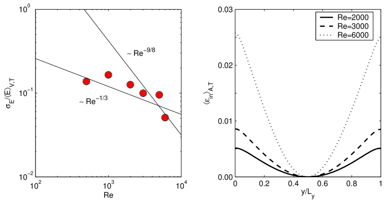
Figure 1: Left: Ratio of standard deviation of the kinetic energy fluctuations, $\sigma_{E}$, and the time average, $\langle E\rangle_{T}=\langle{\bf u}^{2}\rangle_{V,T}/2$, versus Reynolds number, $Re$. Solid lines indicate the power laws with the corresponding exponents. Right: Mean energy injection rate averaged in planes $A=[0,L_{x}]\times[0,L_{z}]$ at fixed $y$ and in time, $\langle\epsilon_{in}\rangle_{A,T}$, as a function of the shear direction $y$. Reynolds numbers are indicated in the legend. The particular kind of steady forcing gives rise to a $y$-dependent profile for the mean energy injection rate.

The variances of the fluctuations in the kinetic energy are shown for different values of the Reynolds number in Fig. 1. In addition to the volume average $\langle\cdot\rangle_{V}$ we will also use averages over planes at fixed $y$ and over time or combinations of spatial and temporal averages which are thought as statistical ensemble averages. Those averages will be indicated by $\langle\cdot\rangle_{A}$ and $\langle\cdot\rangle_{T}$, respectively. The fluctuations of volume averaged kinetic energy (left panel of Fig. 1) decrease with increasing Reynolds number. This is an indication that the increasing number of degrees of freedom that become dynamically active with increasing Reynolds number tend to average out. In quantitative terms the number of active Fourier modes outside the viscous subrange (i.e. with wave lengths exceeding the Kolmorgorov scale $\eta_{K}=(\nu^{3}/\epsilon)^{1/4}$) is roughly $N\sim(L/\eta_{K})^{3}\sim Re^{9/4}$ [17], so that, assuming a law of large numbers, we might expect $\sigma_{E}\sim N^{-1/2}\sim Re^{-9/8}$. Experiments in a closed swirling turbulent flow indicated a slope $\sim Re^{-1/3}$ [5]. For the Reynolds number range accessible in our simulations no definite conclusion on either scaling can be drawn.

For the applied volume forcing the flow is not homogeneous in the shear direction, as indicated by the variations of average energy uptake with position in shear direction (right panel of Fig. 1). It is homogeneous in the downstream and the spanwise direction, so that for all statistical measures we can collect in one ensemble all points in the $x$-$z$-planes for fixed shear coordinate $y$.

The higher energy content of the largest scales and the prevalence of large coherent structures in shear flows [18] suggest that the energy uptake is dominated by large scale flows. In shear flows, the predominant structures are downstream vortices and streamwise streaks. One such event that is connected with a negative energy injection rate is shown in Fig. 2. We do observe fluid moving coherently into the opposite direction to the mean flow $\langle u_{x}\rangle_{A,T}(y)$ which is plotted in the lower right panel of Fig. 2.

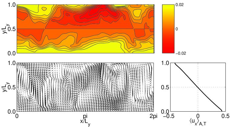
Figure 2: Snapshot of the velocity field and the corresponding energy injection rate field at fixed position $z_{0}/L_{y}=\pi$ for the run with $Re=6000$. The upper panel shows $\epsilon_{in}$ and the lower left panel shows $u_{x}$ and $u_{y}$ in a vector plot. The mean flow profile $\langle u_{x}\rangle_{A,T}(y)$ is indicated in the lower right. Clearly, the dark regions with negative $\epsilon_{in}$ conincide with regions where the fluid moves coherently opposite to the mean flow.

3 Statistical analysis of the energy injection rate

The energy input can be large, both positive and negative, but it cannot be arbitrarily large. Its volume average, $\epsilon_{in}(t)$, can be related to the rms velocity fluctuations by a Cauchy-Schwartz inequality

$$|\langle\epsilon_{in}(t)\rangle_{T}|\leq\left\langle\langle u_{x}^{2}\rangle_{V}^{1/2}\langle F_{x}^{2}\rangle_{V}^{1/2}\right\rangle_{T}=\frac{\nu\pi^{2}U_{0}}{\sqrt{2}L_{y}^{2}}\langle u_{x,rms}\rangle\,.$$ (6)

Fluctuations exceeding the external velocity scale $U_{0}$ are extremely unlikely, so that $\epsilon_{in}$ is bounded by $\sim U_{0}^{2}$. The local energy injection rate can be estimated using the maximum norm, with a similar bound $\sim U_{0}^{2}$, but a different prefactor. For the numerical simulations both bounds turned out to be much too crude and much larger than both the maximal and the rms fluctuations of the downstream velocity. These bounds would thus become effective in the far tails of the probability distribution only.

We focus on the fluctuations of the instantaneous, pointwise energy injection $\epsilon_{in}({\bf x},t)$. We expect that any kind of spatial or temporal average over regions and times longer than the corresponding correlation lengths and times would push the distributions closer to Gaussian shape. It is interesting to note that this does not seem to be the case in [4, 5]. But even there an instantaneous and local distribution should provide a more sensitive measure of possible deviations from a Gaussian shape. Since our system is invariant under translation in downstream and spanwise direction, but not in the normal direction, we study the distributions for planes parallel to the bounding surfaces separately. The probability density functions of the energy input rate in units of its ensemble average, $\langle\epsilon_{in}\rangle_{V,T}$, and for different positions between the plates are shown in Fig. 3.

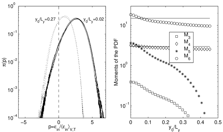
Figure 3: Statistics of energy uptake for different vertical positions in the shear layer. Left: Probability density function (PDF) of the energy input rate. The statistics is based on about 100 turbulent snapshots separated in time by 1.5 large eddy turnover times; it contains about $6\times 10^{8}$ data points. The PDF’s are shown for three different Reynolds numbers, $Re=3000$, $5000$ and $6000$ and the $y_{0}$ values of the fixed planes are indicated in the figure. Right: Normalized moments of $\epsilon_{in}$ versus position $y_{0}/L_{y}$ of fixed plane. Values for a Gaussian distribution, $M_{4}=3$ and $M_{6}=15$, are indicated by solid lines. Reynolds number was 6000.

The collapse of the PDF’s for different Reynolds numbers, rescaled by the volume averages, indicates a universality of the fluctuations of large scale injection (left panel of Fig. 3), as also observed in experiment [5, 7]. The PDF we find is similar to the one measured in [7] and much closer to Gaussian shape than the one in [5]. As a measure of deviations we determine the normalized and centered moments $M_{n}=\langle(p-\langle p\rangle_{A,T})^{n}\rangle/\langle(p-\langle p\rangle_{A,T})^{2}\rangle^{n/2}$ where $\langle(p-\langle p\rangle_{A,T})^{n}\rangle=\int(p-\langle p\rangle_{A,T})^{n}\pi(p)\,\mbox{d}p$ and $p=\epsilon_{in}/\langle\epsilon_{in}\rangle_{V,T}$. In particular, the ones for $n=4$ and $n=6$ differ from the Gaussian values of $3$ and $15$ which are indicated by solid lines in the right panel of Fig. 3. However, the PDF also changes when going from the free-slip side planes at $y_{0}/L_{y}=0$ towards the center at $y_{0}/L_{y}=1/2$: the odd moments are smaller near the center, indicating a more symmetric PDF (see right panel of Fig. 3). The PDF is closest to Gaussian here.

We next turn to the logarithm of the ratio of the probabilities for positive and negative injection rates, $\log[\pi(p)/\pi(-p)]$, where $p$ is again a particular value of the dimensionless instantaneous and local dissipation, $\epsilon_{in}({\bf x},t)/\langle\epsilon_{in}\rangle_{V,T}$. In Fig. 4 we show

$$C_{0}(p)=\frac{1}{p}\log\left[\frac{\pi(p)}{\pi(-p)}\right]\,.$$ (7)

A constant $C_{0}$ indicates a linear exponential relation between the probabilities of positive and negative energy injection.

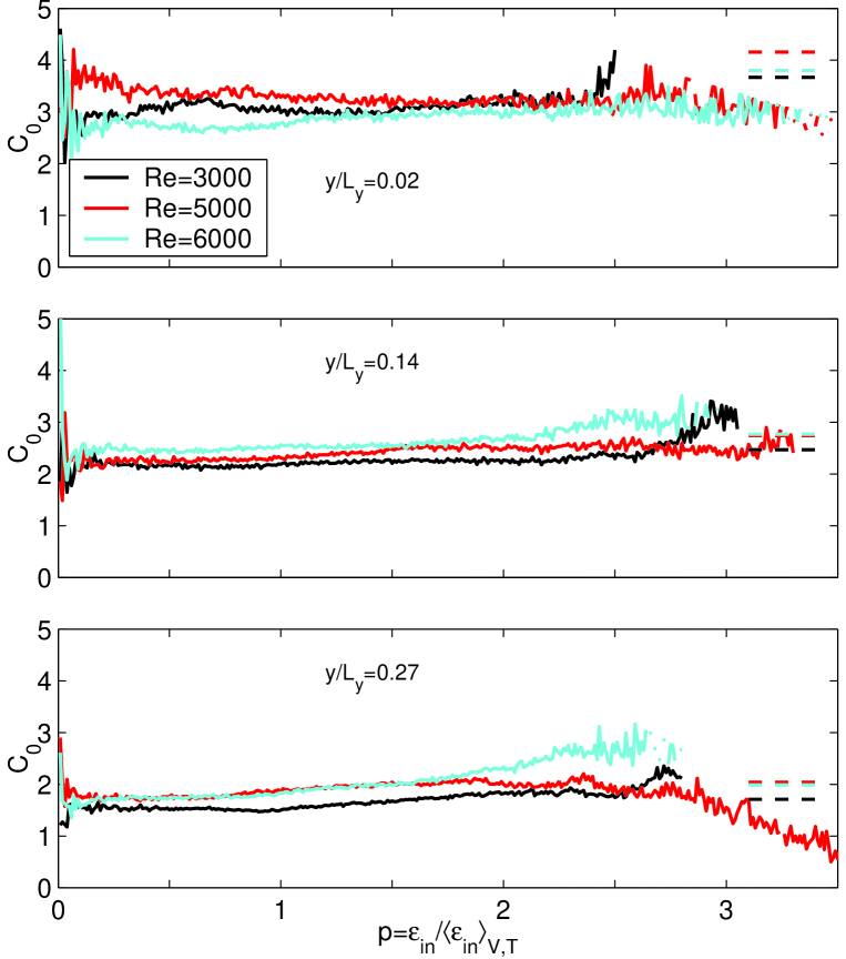
Figure 4: Test of the linearity of the logarithmic ratio as suggested by Eq. (7). The stronger oscillations for very small $p$ arise due to the amplification of small wiggles on the PDF $\pi(p)$ there. The linear slope is fairly independent of $Re$. Data are as in Fig. 3. The dashed lines on the far right indicate the values of $C_{0}$ obtained from Eq. (9).

As is well known the slope $C_{0}$ can be related to the mean and the variance in a Gaussian model for the fluctuations. Clearly the logarithmic ratio of the probability density functions is then automatically linear. If the distribution has the form

$$\pi(p)=N\exp(-(p-\overline{p})^{2}/2\sigma^{2})\,,$$ (8)

with normalization factor $N$, then

$$C_{0}=2\frac{\overline{p}}{\sigma^{2}}=2\frac{\langle\epsilon_{in}\rangle_{A,T}\langle\epsilon_{in}\rangle_{V,T}}{\langle\epsilon_{in}^{2}\rangle_{A,T}-\langle\epsilon_{in}\rangle_{A,T}^{2}}\,.$$ (9)

In Fig. 4, we have also indicated the $C_{0}$ value as given by (9) by dashed lines. For the PDF close to the center of the flow this estimate agrees with the value from the PDF of the data, but near the side planes deviations become visible. Here the strength of energy input is largest on average and coherent flow structures are most prominent. In all cases our $C_{0}$ is larger than unity. A $C_{0}$ larger than unity was also found in Farago’s model of Brownian particle motion where probabilities of time averaged energy injection rates were considered [11].

4 Concluding remarks

We have studied the fluctuations of the energy injection rate in a turbulent shear flow for various Reynolds numbers. The mean value of the energy input rate and the shape of its probability distribution varies across the shear flow. The results do not depend much on the Reynolds number and the probability density functions collapse when rescaled by the mean value of $\epsilon_{in}$. The probabilities for positive and negative energy injection are exponentially related over a range of more than twice the mean values. However, the constant in the exponent varies across the layer. Thus, while there are some indications for an exponential relation between positive and negative energy uptake, the quantitative behaviour depends on the position across the layer.

It is still an open, but interesting, question whether the energy injection rate (smoothed in time or not) can be considered as a macroscopic substitute for the entropy production rate, and whether fluctuation relations for it can be found. As mentioned in the introduction, the Navier-Stokes equation is perhaps closest in its global features to the Brownian particle studied by Farago [11]. That model predicts a crossover to another slope for large energy uptake, but the statistical uncertainties in our numerical data are too large to study this. Other systems that might provide guidance for what to expect in the fluctuation statistics are thermostatted Lorentz gases where time reversibility is broken by a magnetic field [19].

Further avenues worth exploring include the relation between coherent structures and energy uptake or energy blocking (as in Fig. 2), and the implications for backscatter effects in turbulent flows, i.e., the phenomenon that locally energy does not cascade down to smaller but up to larger scales. This might be important for subgrid-scale modelling within large-eddy simulations [20].

Acknowledgements

We thank J. Davoudi, J. R. Dorfman, G. Gallavotti, W. I. Goldburg, W. Losert, L. Rondoni, T. Tel and J. Vollmer for useful discussions. The computations were done on a Cray SV1ex at the John von Neumann-Institut für Computing at the Forschungszentrum Jülich and we are grateful for their support. This work was also supported by the Deutsche Forschungsgemeinschaft.

References

- [1] U. Frisch, Turbulence, Cambridge University Press, Cambridge 1995.
- [2] S. Ciliberto and C. Laroche, J. Phys. IV France 8, (1998) 215.
- [3] W. I. Goldburg, Y. Y. Goldschmidt, and H. Kellay, Phys. Rev. Lett. 87, (2001) 245502.
- [4] S. T. Bramwell, P. C. W. Holdsworth and J.-F. Pinton, Nature 396, (1998) 552.
- [5] J.-F. Pinton, P. C. W. Holdsworth and R. Labbé, Phys. Rev. E 60, (1999) R2452.
- [6] A. Noullez and J.-F. Pinton, Eur. Phys. J. B 28, (2002) 231.
- [7] J. H. Titon and O. Cadot, Phys. Fluids 15, (2003) 625.
- [8] D. J. Evans, E. G. D. Cohen and G. P. Moriss, Phys. Rev. Lett. 71, (1993) 2401.
- [9] G. Gallavotti and E. G. D. Cohen, Phys. Rev. Lett. 74, (1995) 2694; J. Stat. Phys. 80, (1995) 931.
- [10] J. Vollmer, Phys. Rep. 372, (2002) 131.
- [11] J. Farago, J. Stat. Phys. 107, (2002) 781.
- [12] Z.-S. She and E. Jackson, Phys. Rev. Lett. 70, (1993) 1255.
- [13] L. Rondoni and E. Segre, Nonlinearity 12, (1999) 1471.
- [14] G. Gallavotti, L. Rondoni and E. Segre, Lyapunov spectra and nonequilibrium ensembles equivalence in 2D fluid mechanics, preprint (2002).
- [15] S. Aumaître, S. Fauve, S. McNamara and P. Poggi, Eur. Phys. J. B 19, (2001) 449.
- [16] J. Schumacher and B. Eckhardt, Phys. Rev. E 63, (2001) 046307.
- [17] L. D. Landau and E. M. Lifschitz, Course in Theoretical Physics: Fluid Mechanics, Pergamon Press, Oxford, 1987.
- [18] J. Schumacher and B. Eckhardt, Europhys. Lett. 52, (2000) 627.
- [19] M. Dolowschiák and Z. Kovács, Phys. Rev. E 66, (2002) 066217.
- [20] M. Lesieur and O. Metais, Annu. Rev. Fluid Mech. 28, (1996) 45.