Pulsation and Precession of the Resonant Swinging Spring

Abstract

When the frequencies of the elastic and pendular oscillations of an elastic pendulum or swinging spring are in the ratio two-to-one, there is a regular exchange of energy between the two modes of oscillation. We refer to this phenomenon as pulsation. Between the horizontal excursions, or pulses, the spring undergoes a change of azimuth which we call the precession angle. The pulsation and stepwise precession are the characteristic features of the dynamics of the swinging spring.

The modulation equations for the small-amplitude resonant motion of the system are the well-known three-wave equations. We use Hamiltonian reduction to determine a complete analytical solution. The amplitudes and phases are expressed in terms of both Weierstrass and Jacobi elliptic functions. The strength of the pulsation may be computed from the invariants of the equations. Several analytical formulas are found for the precession angle.

We deduce simplified approximate expressions, in terms of elementary functions, for the pulsation amplitude and precession angle and demonstrate their high accuracy by numerical experiments. Thus, for given initial conditions, we can describe the envelope dynamics without solving the equations. Conversely, given the parameters which determine the envelope, we can specify initial conditions which, to a high level of accuracy, yield this envelope.

url]http://www.maths.tcd.ie/$\sim$plynch

url]http://www.maths.tcd.ie/$\sim$houghton

1 Introduction

The present work is concerned with the three-dimensional motion of the elastic pendulum or swinging spring in the case of resonance. It continues the investigation described in previous studies by Lynch [13] and by Holm and Lynch [9]. In particular, the exchange of energy between quasi-vertical and quasi-horizontal oscillations and the stepwise precession of the swing plane are investigated.

When the ratio of the normal mode frequencies of the spring is 2:1, a resonance occurs, in which energy is transferred periodically between vertical and horizontal oscillations. The first study of this resonance was that of Vitt and Gorelik [17]. We refer to the regular exchange phenomenon as pulsation. The motion has two distinct characteristic times, that of the fast oscillations and that of the slow pulsation envelope. As the oscillations change from horizontal to vertical and back again, it is observed that each horizontal excursion or pulse is in a different direction. We call this change in azimuth the precession angle. The motion thus has three components: oscillation (fast), pulsation (slow) and precession (slow), closely analogous to the rotation (fast), nutation (slow) and precession (slow) of a spinning top [3].

We consider two complementary questions, one direct and one inverse:

• Given initial conditions, can we describe the envelope dynamics without solving the equations?

• Given the parameters which determine the envelope, can we specify initial conditions which yield this envelope?

We provide a complete answer to Question 1. Analytical expressions are derived for the pulsation amplitude, precession angle and period in terms of the invariants of the motion. We also develop accurate approximate expressions for the pulsation amplitude and precession angle. Thus, the envelope dynamics may be deduced from the initial conditions. Question 2 is more recondite, but we can give a positive answer for the physically interesting case of strong pulsation. We derive approximate expressions for the angular momentum and Hamiltonian in terms of the pulsation amplitude and precession angle. Initial conditions can then be determined which yield the desired envelope to a good level of approximation.

We briefly outline the contents of the paper below. When the amplitude is small, the Lagrangian may be approximated to cubic order. When it is averaged over the fast oscillation time, a set of equations for the envelope amplitudes is obtained. These modulation equations, the three-wave equations, are presented in §2. They are found to have three independent constants of motion and are therefore completely integrable. Small-amplitude perturbations about steady-state solutions are studied in §3, and a crude estimate of the precession angle is obtained. The general solution of the three-wave equations for finite-amplitude motions is derived in §4. The amplitudes are expressed in terms of elliptic functions and the phase angles as elliptic integrals. Analytical expressions for the stepwise precession of the swing-plane are then derived.

Recently, Dullin et al. [5] constructed a canonical transformation in which the angle of the swing plane is a coordinate in an action-angle system. They showed that the precession angle is one of the two rotation numbers of the invariant tori of the integrable system. They obtained a simple equation for the precession angle by approximating an elliptic integral. They proved analytically that the resonant swinging spring has monodromy and concluded that the system provides a clear physical demonstration of this phenomenon.

Several approximate expressions for the precession angle, involving only elementary functions, are obtained in §5. One of these is equivalent to the formula reported in [5]. The approximate solutions are compared to the values obtained from the analytical expression, and are found to give remarkably accurate results. The intensity of the pulsation envelope is determined by solving a cubic equation whose coefficients are defined by the invariants. Thus, the direct question is fully answered, in the affirmative.

To answer the inverse question, we assume the pulsation amplitude and precession angle are given and derive expressions for the invariants. From these, appropriate initial conditions are easily determined. The expression for the precession angle is easily inverted. To obtain an invertible expression for the pulsation amplitude, we approximate the cubic by a quadratic, and obtain in §6 simple approximate expressions for the angular momentum and Hamiltonian. These approximations may be used to control the envelope dynamics by an appropriate choice of initial conditions.

In the concluding section, §7, we present a schematic diagram which shows the qualitative dependence of the envelope motion on the values of the invariants. This allows us to determine, at a glance, the general character of the solution for given values of the constants of motion. Several important special solutions are indicated on the diagram.

2 The Dynamical Equations

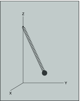
Figure 1: The swinging spring. Cartesian coordinates are used, with the origin at the point of stable equilibrium of the bob. The pivot is at point $(0,0,\ell)$.

The physical system under investigation is an elastic pendulum, or swinging spring, consisting of a heavy mass suspended from a fixed point by a light spring and moving under gravity, $g$ (Fig. 1). We assume an unstretched length $\ell_{0}$, length $\ell$ at equilibrium, spring constant $k$ and mass $m$. The Lagrangian, approximated to cubic order in the amplitudes, is

$$L=\textstyle\frac{1}{2}\left(\dot{x}^{2}+\dot{y}^{2}+\dot{z}^{2}\right)-\textstyle\frac{1}{2}\left[\omega_{R}^{2}(x^{2}+y^{2})+\omega_{Z}^{2}z^{2}\right]+\textstyle\frac{1}{2}\lambda(x^{2}+y^{2})z\,,$$ (1)

where $x$, $y$ and $z$ are Cartesian coordinates centered at the point of equilibrium, $\omega_{R}=\sqrt{g/\ell}$ is the frequency of linear pendular motion, $\omega_{Z}=\sqrt{k/m}$ is the frequency of its elastic oscillations and $\lambda=\ell_{0}\omega_{Z}^{2}/\ell^{2}$. The equations of motion in cartesian, spherical and cylindrical coordinates may be found in [13]. There are two constants of the motion, the total energy and the angular momentum about the vertical, and the system is not integrable. Its chaotic motions have been studied by many authors (see Refs. in [14]).

2.1 The Time-averaged Equations

We confine attention to the resonant case $\omega_{Z}=2\omega_{R}$ and apply the averaged Lagrangian technique. The solution is assumed to be of the form

$$x = \Re\{a(t)\exp(i\omega_{R}t)\}\,,$$ (2)

$$y = \Re\{b(t)\exp(i\omega_{R}t)\}\,,$$ (3)

$$z = \Re\{c(t)\exp(2i\omega_{R}t)\}\,.$$ (4)

The coefficients $a(t)$, $b(t)$ and $c(t)$ are assumed to vary on a time scale which is much longer than the time-scale of the oscillations, $\tau=1/\omega_{R}$. The Lagrangian is averaged over this time, yielding

$$\langle L\rangle=\textstyle\frac{1}{2}\omega_{R}\Big{[}\Im\{\dot{a}a^{*}+\dot{b}b^{*}+2\dot{c}c^{*}\}+\Re\{\kappa(a^{2}+b^{2})c^{*}\}\Big{]}\,,$$

where $\kappa=\lambda/(4\omega_{\rm R})$. The resulting Euler-Lagrange equations are the modulation equations for the envelope dynamics:

$$i\dot{a} = \kappa a^{*}c\,,$$ (5)

$$i\dot{b} = \kappa b^{*}c\,,$$ (6)

$$i\dot{c} = \textstyle{\frac{1}{4}}\kappa(a^{2}+b^{2})\,.$$ (7)

2.2 The three-wave equations

We now transform to new variables

$$A=\textstyle\frac{1}{2}\kappa(a+ib)\,,\quad B=\textstyle\frac{1}{2}\kappa(a-ib)\,,\quad C=\kappa c\,.$$ (8)

Then the equations for the envelope dynamics take the form

$$i\dot{A} = B^{*}C\,,$$ (9)

$$i\dot{B} = CA^{*}\,,$$ (10)

$$i\dot{C} = AB\,,$$ (11)

These three equations for the slowly-varying complex amplitudes $A$, $B$ and $C$ are the three-wave equations. The relevance of these equations in various physical contexts is discussed in [9]. They govern quadratic wave resonance in fluids and plasmas. Their application to resonant Rossby wave triads is considered in [15]. In Appendix A, we show that they are a special case of the Nahm equations which are used to construct soliton solutions in certain particle field theories. For further references to the three-wave equations and a discussion of their properties see [2].

The three-wave equations conserve the following three quantities:

$$H = \textstyle\frac{1}{2}(ABC^{*}+A^{*}B^{*}C)=\Re\{ABC^{*}\}\,,$$ (12)

$$N = |A|^{2}+|B|^{2}+2|C|^{2}\,,$$ (13)

$$J = |A|^{2}-|B|^{2}\,.$$ (14)

The equations are completely integrable. The following positive-definite combinations of $N$ and $J$ are physically significant:

$$N_{+}\equiv\textstyle\frac{1}{2}(N+J)=|A|^{2}+|C|^{2}\,,\qquad N_{-}\equiv\textstyle\frac{1}{2}(N-J)=|B|^{2}+|C|^{2}\,.$$

These combinations are known as the Manley-Rowe relations. Together with the Hamiltonian $H$, they provide three independent constants of the motion. We note that $H$ is invariant under the symmetry transformations

$$(A,B,C) \rightarrow (Ae^{i\chi},Be^{-i\chi},C)\,,$$ (15)

$$(A,B,C) \rightarrow (Ae^{i\chi},B,Ce^{i\chi})\,,$$ (16)

$$(A,B,C) \rightarrow (A,Be^{i\chi},Ce^{i\chi})\,.$$ (17)

These symmetries are associated, via Noether’s theorem, with the three invariants $\big{\{}J,N_{+},N_{-}\big{\}}$. Any two of the transformations generate the third. This reflects the inter-dependence of $J$, $N_{+}$ and $N_{-}$.

2.3 Reduction of the system

To reduce the system for $H\neq 0$, we express the amplitudes in polar form:

$$A = |A|\exp(i\xi)\,,$$ (18)

$$B = |B|\exp(i\eta)\,,$$ (19)

$$C = |C|\exp(i\gamma)\,.$$ (20)

In general, the phases of $A$, $B$ and $C$ are not periodic. However, $\zeta=\gamma-(\xi+\eta)$ is periodic. The Hamiltonian may be written

$$H=|A||B||C|\cos\zeta\,.$$

The amplitude $|C|$ will be obtained in closed form in terms of elliptic functions. Once $|C|$ is known, $|A|$ and $|B|$ follow immediately from the Manley-Rowe relations

$$|A|=\sqrt{N_{+}-|C|^{2}}\,,\qquad|B|=\sqrt{N_{-}-|C|^{2}}\,.$$

The phases $\xi$ and $\eta$ may now be determined. Using the three-wave equations (9)–(11) together with equations (18)–(20), we find

$$\dot{\xi}=-\frac{H}{|A|^{2}}\,,\qquad\dot{\eta}=-\frac{H}{|B|^{2}}\,,$$ (21)

so that $\xi$ and $\eta$ can be obtained by quadratures. Finally, $\zeta$ is determined unambiguously by

$$\frac{d|C|^{2}}{dt}=-2H\tan\zeta\qquad{\rm and}\qquad H=|A||B||C|\cos\zeta\,.$$ (22)

It also follows from (21) and (22) that

$$\dot{\zeta}={H}\left(\frac{1}{|A|^{2}}+\frac{1}{|B|^{2}}-\frac{1}{|C|^{2}}\right)\,.$$ (23)

The phase of $C$ follows immediately, $\gamma=\xi+\eta+\zeta$, and we can then reconstruct the complete solution using (18)–(20).

2.4 The equation for $|C|^{2}$

Figure 2: Polynomial $\Phi_{0}$ as a function of $|C|^{2}$.

From the equation (11) for $\dot{C}$, and its complex conjugate we get

$$\frac{d|C|^{2}}{dt}=2\Im\{ABC^{*}\}\,.$$ (24)

Using the definition of the Hamiltonian, it follows that

$$|A|^{2}|B|^{2}|C|^{2}=H^{2}+[\Im\{ABC^{*}\}]^{2}\,.$$

Applying this to the square of (24) and using the definitions of the Manley-Rowe quantities immediately yields an equation for $|C|^{2}$ alone:

$$\left(\frac{d|C|^{2}}{dt}\right)^{2}=4\Big{[}(N_{+}-|C|^{2})(N_{-}-|C|^{2})|C|^{2}-H^{2}\Big{]}\,.$$ (25)

We define the cubic polynomial $\Phi_{0}(|C|^{2})$ (plotted in Fig. 2) by

$$\Phi_{0}(|C|^{2})=(N_{+}-|C|^{2})(N_{-}-|C|^{2})|C|^{2}\,.$$ (26)

Then the right hand side of (25) may be written $4[\Phi_{0}(|C|^{2})-H^{2}]$. For small $H^{2}$, this cubic has three positive real roots. If these roots, in descending order of magnitude, are denoted $C_{1}^{2}$, $C_{2}^{2}$ and $C_{3}^{2}$, it follows that

$$0\leq C_{3}^{2}\leq C_{2}^{2}\leq N_{-}\leq\textstyle\frac{1}{2}N\leq N_{+}\leq C_{1}^{2}\leq N\,.$$ (27)

(We have assumed without loss of generality that $J\geq 0$). In the case of equality of roots, the solution may be obtained in terms of elementary functions. We assume in general that this is not so and solve for $|C|^{2}$ in terms of elliptic functions. However, before doing this, we investigate perturbation motion about steady solutions.

3 Small-Amplitude Modulation of Steady States

We consider the case where the variations of the amplitudes about their mean values are small. This enables us to make additional approximations and derive simple estimates of the pulsation period and rate of precession. From these two quantities, the precession angle follows immediately.

3.1 Steady State Motion

We first consider solutions for which the amplitudes $|A|$, $|B|$ and $|C|$ are constant. The simplest cases are where the phases are also constant; then the three-wave equations become

$$B^{*}C=CA^{*}=AB=0\,,$$

which give three particular solutions

$$(i)\qquad A=A_{0}\,,\quad B=C=0\,;$$

$$(ii)\qquad B=B_{0}\,,\quad C=A=0\,;$$

$$(iii)\qquad C=C_{0}\,,\quad A=B=0\,.$$

The first two solutions correspond to conical motions: the bob moves in a circle, clockwise or anti-clockwise, while the spring traces out a cone. These solutions are stable to small perturbations. The third particular case represents purely vertical oscillations; this motion is unstable [13].

More generally, from (22), constancy of the amplitudes implies $\zeta=\gamma-(\xi+\eta)=0$ so that $H=|A||B||C|$, and the three-wave equations become

$$-|A|\dot{\xi} = |B||C|$$

$$-|B|\dot{\eta} = |C||A|$$ (28)

$$-|C|\dot{\gamma} = |A||B|\,.$$

Differentiating (25), a simple algebraic manipulation yields

$$|C|^{2}=C_{0}^{2}\equiv\frac{1}{6}\left(2N-\sqrt{N^{2}+3J^{2}}\right)$$ (29)

The other amplitudes are given by

$$|A|^{2} = A_{0}^{2}\equiv\frac{1}{6}\left[(N+3J)+\sqrt{N^{2}+3J^{2}}\right]$$

$$|B|^{2} = B_{0}^{2}\equiv\frac{1}{6}\left[(N-3J)+\sqrt{N^{2}+3J^{2}}\right]$$

These solutions are the elliptic-parabolic modes (EP-modes) studied by Lynch [13]. The precession rate is given by $\Omega\equiv\dot{\phi}=\textstyle\frac{1}{2}(\dot{\xi}-\dot{\eta})$ [9]. From (28) it follows that

$$\Omega=\frac{JC_{0}^{2}}{2H}\,.$$ (30)

For $J=0$ we have planar motion with

$$|C|^{2}=\frac{N}{6}\,,\qquad|A|^{2}=|B|^{2}=\frac{N}{3}\,.$$

These are the cup-like and cap-like solutions of Vitt and Gorelik [17].

3.2 Perturbation about Elliptic-Parabolic Motion

We consider small deviations about the steady EP-mode solutions. We write $|C|^{2}=C_{0}^{2}+\epsilon$ where $C_{0}^{2}$ is given by (29) and $|\epsilon|\ll C_{0}^{2}$. Then, if (25) is differentiated and nonlinear terms in $\epsilon$ are omitted, we obtain

$$\frac{d^{2}\epsilon}{dt^{2}}+\left(2\sqrt{N^{2}+3J^{2}}\right)\epsilon=0\,.$$ (31)

The solution is $\epsilon(t)=\epsilon(0)\cos\omega_{\rm P}t$, an oscillation about $C_{0}^{2}$ with the pulsation frequency

$$\omega_{\rm P}=\sqrt{2}{\root 4 \of{N^{2}+3J^{2}}}\,.$$ (32)

For the EP-modes, the horizontal projection is an ellipse precessing at a constant rate $\Omega$. The perturbation is a pulsating motion, with sinusoidal time variation, in which the major and minor axes of the ellipse alternately expand and contract with period $T_{\rm P}=2\pi/\omega_{\rm P}$. The area of the ellipse is proportional to $J$ and remains constant [9]. It is straightforward to derive expressions in terms of elementary functions for the remaining amplitudes and the phases, but they are not required to determine the precession angle.

We note from (32) that $\sqrt{2N}\leq\omega_{\rm P}\leq 2\sqrt{2N}$. From the precession rate and the pulsation frequency, the precession angle follows immediately:

$$\Delta\phi=\Omega T_{\rm P}\,.$$

Using (29), (30) and (32), this gives us

$${\Delta\phi=\frac{JC_{0}^{2}}{2H}\frac{2\pi}{\omega_{\rm P}}=\frac{\pi}{3}\left(\frac{J}{\sqrt{8}H}\right)\left[\frac{2N-\sqrt{N^{2}+3J^{2}}}{\root 4 \of{N^{2}+3J^{2}}}\right]\,.}$$ (33)

For small angular momentum $J\ll N$, the term in square brackets is close to $\sqrt{N}$ and

$$\Delta\phi\approx\frac{\pi}{3}\left(\frac{J\sqrt{N}}{\sqrt{8}H}\right)\,.$$ (34)

4 Analytical Solution of the Three-wave Equations

4.1 Solution in Weierstrass Elliptic Functions

We now derive an explicit analytical solution for $|C|^{2}$, valid for finite amplitudes. The solutions for $|A|^{2}$ and $|B|^{2}$ follow immediately from the Manley-Rowe relations. Then (21) are integrated for the phases. The integrals turn out to be similar to those occurring for the spherical pendulum, so the approach of Whittaker [18] applies. The required properties of the Weierstrass elliptic functions are given in Whittaker and Watson [19], Ch. 20 and in Lawden [12], Ch. 6 (see also Abramowitz and Stegun [1], Gradshteyn and Ryzhik [7] and Byrd and Friedman [4]).

4.1.1 Solution for the amplitudes

The quadratic term on the right of (25) is removed by a simple transformation $u=|C|^{2}/N-1/3$ and $\tau=\sqrt{N}t$. Then we obtains

$$\left(\frac{d\,u}{d\tau}\right)^{2} = 4u^{3}-g_{2}u-g_{3}$$ (35)

$$= 4(u-e_{1})(u-e_{2})(u-e_{3})\,.$$

This is the standard form of the equation for Weierstrass elliptic functions. The constants $g_{2}$ and $g_{3}$, called the invariants, are given by

$$g_{2}=\left(\frac{1}{3}+\frac{J^{2}}{N^{2}}\right)\,,\qquad g_{3}=\left(-\frac{1}{27}+\frac{J^{2}}{3N^{2}}+\frac{4H^{2}}{N^{3}}\right)\,.$$

For small $H^{2}$, the discriminant $\Delta=g_{2}^{3}-27g_{3}^{2}$ is positive and the three roots are real. This is the case of physical interest, and we assume the roots of the cubic are ordered so that $e_{1}>e_{2}>e_{3}$. Note that $e_{1}+e_{2}+e_{3}=0$. The general solution of (35) is

$$u=\wp(\tau+\alpha)$$

where $\alpha$ is an arbitrary (complex) constant. The function $\wp(z)$ is defined by

$$\wp(z)=\frac{1}{z^{2}}+{\sum_{m,n}}^{\prime}\left\{\frac{1}{(z-2m\omega_{1}-2n\omega_{2})^{2}}-\frac{1}{(2m\omega_{1}+2n\omega_{2})^{2}}\right\}$$ (36)

where the summation is over all integral $m$, $n$ except $m=n=0$. It has poles on the real line and is doubly periodic: $\wp(z+2m\omega_{1}+2n\omega_{2})=\wp(z)$ for all integers $m$ and $n$. The difficult problem of determining $\omega_{1}$ and $\omega_{2}$ from the invariants is discussed in §21.73 of [19]. The quantity $\omega_{3}$ is defined by requiring $\omega_{1}+\omega_{2}+\omega_{3}=0$. It may be shown that

$$\wp(\omega_{1})=e_{1}\,\qquad\wp(\omega_{2})=e_{2}\,\qquad\wp(\omega_{3})=e_{3}\,.$$ (37)

In the present case, $\omega_{1}$ is real and $\omega_{3}$ is pure imaginary (explicit expressions are given below). On the real line, $\wp(z)$ is real, with values in the range $[e_{1},+\infty)$. On the line $z=\omega_{3}+x$ it takes real values in the interval $[e_{3},e_{2}]$. Moreover, as $z$ varies along the edge of the rectangle from $0$ to $\omega_{1}$ to $\omega_{1}+\omega_{3}(=-\omega_{2})$ to $\omega_{3}$ to $0$, $\wp(z)$ is real and decreases monotonically from $+\infty$ to $e_{1}$ to $e_{2}$ to $e_{3}$ to $-\infty$. To satisfy the initial conditions, we choose $\alpha=\omega_{3}-\tau_{0}$, where $\tau_{0}$ is real and may be taken as zero by a suitable choice of time origin. Then $\wp(\tau+\omega_{3})$ is real and oscillates between $e_{3}$ and $e_{2}$. The solution for the amplitude is

$$|C|^{2}=N\left[\textstyle\frac{1}{3}+\wp(\tau+\omega_{3})\right]\,.$$ (38)

The behaviour of the Weierstrass $\wp$-function is shown in Figure 3. For general $z$ it takes complex values. On the line $\Im\{z\}=\omega_{3}$ the function is real with periodic oscillations, as indicated by the heavy lines at the front of the figure.

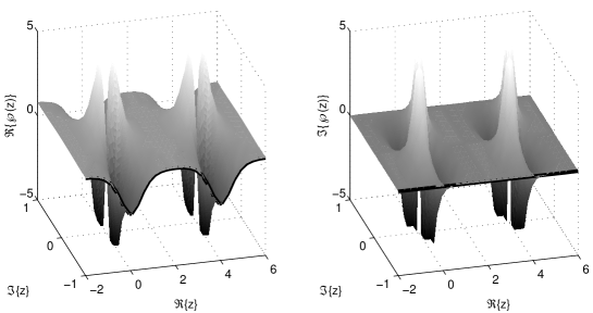
Figure 3: Weierstrass’s $\wp$-function with half-periods $\omega_{1}=2$, $\omega_{3}=i$ on the domain $\{z=x+iy:x\in[-2,+6],y\in[-1,+1]$. Left panel: real part; right panel: imaginary part. Values for $z=x-\omega_{3}$ are plotted as heavy lines. Calculations are based on (36). The function has double poles at $z=2m\omega_{1}+2n\omega_{2}$.

4.1.2 Solution for the phase angles

Weierstrass’s zeta function is defined by

$$\frac{d\mathbf{\zeta}}{dz}=-\wp(z)\,,\qquad\lim_{z\rightarrow 0}\,[\mathbf{\zeta}(z)-z^{-1}]=0\,.$$ (39)

It is quasi-periodic in the sense that

$$\mathbf{\zeta}(z+2\omega_{1})=\mathbf{\zeta}(z)+2\mathbf{\zeta}(\omega_{1})\,.$$ (40)

We note that $\mathbf{\zeta}(z)$ is an odd function of $z$ and will use the relation

$$\omega_{1}\mathbf{\zeta}(\omega_{2})-\omega_{2}\mathbf{\zeta}(\omega_{1})=\textstyle\frac{1}{2}\pi i\,.$$ (41)

The sigma function is defined by

$$\frac{d}{dz}\log\sigma(z)=\mathbf{\zeta}(z)\,,\qquad\lim_{z\rightarrow 0}\,\frac{\sigma(z)}{z}=1\,.$$ (42)

It is also quasi-periodic, such that

$$\sigma(z+2\omega_{1})=-\exp[2\mathbf{\zeta}(\omega_{1})(z+\omega_{1})]\,\sigma(z)\,.$$ (43)

Three other sigma functions may be defined. The relationship between the sigma functions and the Weierstrass $\wp$-function is similar to that between the theta functions and the Jacobi elliptic functions. We will not require these. We will require the identity

$$\frac{\wp^{\prime}(\alpha)}{\wp(z)-\wp(\alpha)}=\mathbf{\zeta}(z-\alpha)-\mathbf{\zeta}(z+\alpha)+2\mathbf{\zeta}(\alpha)$$ (44)

(this follows from a consideration of the poles and zeros of the functions on each side).

The solution (38) leads to a solution for $|A|^{2}$:

$$|A|^{2}=\frac{N+3J}{6}-N\wp(\tau+\omega_{3})\,.$$ (45)

Substituting in the first of (21) we have

$$\sqrt{N}\,\frac{d\xi}{d\tau}=\frac{6H}{6N\wp(\tau+\omega_{3})-(N+3J)}$$

Now we introduce auxiliary constants $\kappa_{\pm}$ defined by

$$\wp(\kappa_{+})=\frac{N+3J}{6N}\equiv e_{+}\,,\qquad\wp(\kappa_{-})=\frac{N-3J}{6N}\equiv e_{-}\,.$$

Using (35), it follows that

$$[\wp^{\prime}(\kappa_{+})]^{2}=[\wp^{\prime}(\kappa_{-})]^{2}=-\left(\frac{4H^{2}}{N^{3}}\right)\,.$$

We must determine which sign for the derivatives should be chosen. From (27) the following sequence of inequalities holds:

$$-\textstyle\frac{1}{3}\leq e_{3}\leq e_{2}\leq e_{-}\leq\textstyle\frac{1}{6}\leq e_{+}\leq e_{1}\leq\textstyle\frac{2}{3}\,.$$ (46)

Since $e_{2}<e_{-}<e_{+}<e_{1}$, it follows that $\kappa_{\pm}$ lie on the line between $\omega_{1}$ and $\omega_{1}+\omega_{3}$, which determines the sign of the derivatives to be $\wp^{\prime}(\kappa_{\pm})=2iH/N^{3/2}$, a positive imaginary number. The equation for $\xi$ thus becomes

$$\frac{d\xi}{d\tau}=\left(\frac{1}{2i}\right)\frac{\wp^{\prime}(\kappa_{+})}{\wp(\tau+\omega_{3})-\wp(\kappa_{+})}$$

Using (44) this may be expressed in terms of zeta functions and using (42) it may be integrated immediately to yield

$$\xi-\xi_{0}=\left(\frac{1}{2i}\right)\left\{\log\left[\frac{\sigma(\tau+\omega_{3}-\kappa_{+})}{\sigma(\tau+\omega_{3}+\kappa_{+})}\right]+2\mathbf{\zeta}(\kappa_{+})\tau\right\}\,.$$ (47)

A similar expression holds for $\eta-\eta_{0}$ with $\kappa_{-}$ replacing $\kappa_{+}$. Thus we obtain the expression for the azimuthal angle $\phi$:

$${\phi-\phi_{0}}=\left(\frac{1}{2i}\right)\left\{[\mathbf{\zeta}(\kappa_{+})-\mathbf{\zeta}(\kappa_{-})]\tau+\frac{1}{2}\log\left[\frac{\sigma(\tau+\omega_{3}-\kappa_{+})}{\sigma(\tau+\omega_{3}+\kappa_{+})}\frac{\sigma(\tau+\omega_{3}+\kappa_{-})}{\sigma(\tau+\omega_{3}-\kappa_{-})}\right]\right\}\,.$$

This is the solution for the azimuth as a function of time. Using the quasi-periodic properties (40) and (43), the change in $\phi$ when $\tau$ varies by $2\omega_{1}$ may be computed:

$$\framebox{$\Delta\phi=-i\omega_{1}\big{(}\mathbf{\zeta}(\kappa_{+})-\mathbf{\zeta}(\kappa_{-})\big{)}+i\mathbf{\zeta}(\omega_{1})(\kappa_{+}-\kappa_{-})$}$$ (48)

This is the desired analytical expression for the pulsation angle.

We note two obvious special cases of (48). When $J=0$ we have $\kappa_{+}=\kappa_{-}$, yielding a zero result for $\Delta\phi$. When $H=0$, we have $\kappa_{+}=\omega_{1}$ and $\kappa_{-}=-\omega_{2}$, so

$$\Delta\phi=-i[\omega_{1}\mathbf{\zeta}(\omega_{2})-\omega_{2}\mathbf{\zeta}(\omega_{1})]=\frac{\pi}{2}\,,$$ (49)

where we have used (41). These two special cases intersect in the homoclinic orbit (with $J=H=0$) which has an infinite transition time.

4.2 Solution in Jacobi Elliptic Functions

While (48) is the analytical solution, it is not immediately obvious how numerical information may be extracted from it. The quantities on the right side are all computable in principle, but at the expense of considerable effort. It is therefore useful to seek an alternative expression, in terms of Jacobi elliptic functions.

4.2.1 Solution for the amplitudes

Recall that with the transformation $u=|C|^{2}/N-1/3$ and $\tau=\sqrt{N}t$, (25) was transformed to (35), which we write again for convenience:

$$\left(\frac{d\,u}{d\tau}\right)^{2}=4(u-e_{1})(u-e_{2})(u-e_{3})\,.$$ (50)

For solutions of physical interest, $H^{2}$ is sufficiently small that the three roots of the cubic are real. Defining the quantities

$$k^{2}=\left(\frac{e_{2}-e_{3}}{e_{1}-e_{3}}\right)\qquad\mbox{and}\qquad\nu^{2}=(e_{1}-e_{3})\,,$$

a further transformation,

$$w=\sqrt{\frac{u-e_{3}}{e_{2}-e_{3}}}\,,\qquad s=\nu\tau\,,$$

brings equation (50) to the standard form

$$\left(\frac{dw}{ds}\right)^{2}=(1-w^{2})(1-k^{2}w^{2})\,.$$ (51)

The solution is $w=\mathrm{sn}(s-s_{0})$, or

$$u=e_{3}+(e_{2}-e_{3})\,\mathrm{sn}^{2}(s-s_{0})$$

where $s_{0}$ is arbitrary. The Jacobi elliptic function $\mathrm{sn}\,s$ has period $4K$, where

$$K=K(k)=\int_{0}^{1}\frac{dw}{\sqrt{(1-w^{2})(1-k^{2}w^{2})}}\,,$$ (52)

so $\mathrm{sn}^{2}(s-s_{0})$ has period $2K$. For definiteness, we set $s_{0}=0$, which means choosing the origin of time where the solution has a minimum:

$$|C|^{2}=C_{3}^{2}+(C_{2}^{2}-C_{3}^{2})\,\mathrm{sn}^{2}(\nu\sqrt{N}t)\,.$$ (53)

Clearly, $|C|$ oscillates between $C_{3}$ and $C_{2}$ with physical period

$$T=2K/\nu\sqrt{N}\,.$$ (54)

The remaining amplitudes, $|A|$ and $|B|$, follow from the Manley-Rowe relations:

$$|A|^{2}={N_{+}-|C|^{2}}\,,\qquad|B|^{2}={N_{-}-|C|^{2}}\,.$$

They have the same period as $|C|$ but vary in anti-phase with it and in phase with each other. We denote the minimum and maximum values of $|A|$ by $A_{3}$ and $A_{2}$, and similarly for $|B|$. Thus

$$N_{+}=A_{3}^{2}+C_{2}^{2}=A_{2}^{2}+C_{3}^{2}\,,\qquad N_{-}=B_{3}^{2}+C_{2}^{2}=B_{2}^{2}+C_{3}^{2}\,.$$

The initial values of the amplitudes (for $s_{0}=0$) are

$$|A(0)|=A_{2}\,,\qquad|B(0)|=B_{2}\,,\qquad|C(0)|=C_{3}\,.$$

We note here an important scaling invariance of the three-wave equations. If the amplitudes are magnified by a constant factor and the time is contracted by the same factor, the form of the equations (9)–(11) is unchanged. Thus, the period of the modulation envelope motion varies inversely with its amplitude. The overall scale may be measured by $\sqrt{N}$ and the inverse dependence of $T$ on this is seen in (54).

The solutions (38) and (53) must be equivalent. This follows from identities relating Weierstrass and Jacobi elliptic functions. The complimentary modulus is defined as $k^{\prime}=\sqrt{1-k^{2}}$, and we write $K^{\prime}=K(k^{\prime})$. The parameters are related by

$$k=\sqrt{\frac{e_{2}-e_{3}}{e_{1}-e_{3}}}\,,\quad k^{\prime}=\sqrt{\frac{e_{1}-e_{2}}{e_{1}-e_{3}}}\,,\quad\omega_{1}=\frac{K}{\sqrt{e_{1}-e_{3}}}\,,\quad\omega_{3}=\frac{iK^{\prime}}{\sqrt{e_{1}-e_{3}}}$$

([7], p. 919). Then we have

$$\wp(z)=e_{3}+\frac{e_{1}-e_{3}}{\mathrm{sn}^{2}(\sqrt{e_{1}-e_{3}}\,z)}$$

But the Jacobi function $\mathrm{sn}(s+iK^{\prime})$ is given in terms of its value on the real line by

$$\mathrm{sn}(s+iK^{\prime})=\frac{1}{k\,\mathrm{sn}\,s}$$

and the equivalence between the two forms of solution follows immediately.

4.2.2 Solution for the phase angles

It remains to determine the phases. Integration of (21) furnishes the angles $\xi$ and $\eta$. We define

$$\gamma_{+}^{2}=\frac{C_{2}^{2}-C_{3}^{2}}{N_{+}-C_{3}^{2}}=\frac{e_{2}-e_{3}}{e_{+}-e_{3}}\,, \lambda_{+}=\frac{H}{\nu\sqrt{N}{A_{2}^{2}}}=\frac{H/N^{3/2}}{\sqrt{e_{1}-e_{3}}(e_{+}-e_{3})}\,,$$

$$\gamma_{-}^{2}=\frac{C_{2}^{2}-C_{3}^{2}}{N_{-}-C_{3}^{2}}=\frac{e_{2}-e_{3}}{e_{-}-e_{3}}\,, \lambda_{-}=\frac{H}{\nu\sqrt{N}{B_{2}^{2}}}=\frac{H/N^{3/2}}{\sqrt{e_{1}-e_{3}}(e_{-}-e_{3})}\,.$$

It follows from (46) that $k^{2}<\gamma_{+}^{2}<\gamma_{-}^{2}<1$. We may now write (21) in the form

$$\frac{d\xi}{ds}=-\frac{\lambda_{+}}{1-\gamma_{+}^{2}\,\mathrm{sn}^{2}s}\,,\qquad\frac{d\eta}{ds}=-\frac{\lambda_{-}}{1-\gamma_{-}^{2}\,\mathrm{sn}^{2}s}\,.$$ (55)

The right sides are the integrands occuring in Legendre’s elliptic integral of the third kind ([1], p. 590). They may be put in standard algebraic form by defining $x=\mathrm{sn}\,s$. Writing

$$\Pi(s,a,k)\equiv\int_{0}^{s}\frac{ds}{1-a\,\mathrm{sn}^{2}s}=\int_{0}^{x}\frac{dx}{(1-ax^{2})\sqrt{(1-x^{2})(1-k^{2}x^{2})}}\,,$$

the solution for $\xi$ becomes

$$\xi-\xi_{0}=-\lambda_{+}\Pi\big{(}s,\gamma_{+}^{2},k\big{)}\,.$$ (56)

There is an analogous solution for $\eta$. The changes in $\xi$ and $\eta$ over a half period $s\in[0,K]$ are

$$\textstyle\frac{1}{2}\Delta\xi=-\lambda_{+}\Pi(\gamma_{+}^{2},k)\,,\qquad\textstyle\frac{1}{2}\Delta\eta=-\lambda_{-}\Pi(\gamma_{-}^{2},k)\,,$$

where the complete elliptic integral is defined as $\Pi(a,k)=\Pi(K,a,k)$. The azimuthal angle of the pendulum is $\phi=\textstyle\frac{1}{2}(\xi-\eta)$. Thus, the change in the azimuth over a full pulsation period is

$$\framebox{$\Delta\phi=-\Big{(}\lambda_{+}\Pi(\gamma_{+}^{2},k)-\lambda_{-}\Pi(\gamma_{-}^{2},k)\Big{)}\,.$}$$ (57)

In Appendix B, an alternative formula (94) is derived from the expression (57), which is structurally similar to (48) obtained above. Using this formula, the limiting cases $\Delta\phi=0$ for $J=0$ and $\Delta\phi=\pi/2$ for $H=0$ are again derived, in agreement with (49).

5 Approximate Formulas for the Precession Angle

We have derived an exact analytical expression for the precession angle, involving elliptic integrals. It is of interest to obtain more convenient approximate formulas, involving only elementary functions. It might be expected that the easiest way to do this would be to approximate (57) directly. However, it turns out that it is easier, and more transparent, to return to the differential equations governing the the system, use them to write down an integral for the precession angle and approximate this integral.

The precession angle is $\phi=\textstyle\frac{1}{2}(\xi-\eta)$. Combining the two components of (21), we obtain

$$\frac{d\phi}{dt}=\frac{JH}{2|A|^{2}|B|^{2}}\,.$$ (58)

Eq. (24) may be written

$$\frac{d|C|^{2}}{dt}=\pm 2\sqrt{|A|^{2}|B|^{2}|C|^{2}-H^{2}}\,.$$ (59)

Taking the quotient of these two equations, we get

$$\frac{d\phi}{d|C|^{2}}=\pm\frac{JH}{4|A|^{2}|B|^{2}\sqrt{|A|^{2}|B|^{2}|C|^{2}-H^{2}}}\,.$$ (60)

The pulsation of the amplitude $|C|$ occurs between $C_{2}$ and $C_{3}$, where $C_{3}^{2}$ and $C_{2}^{2}$ are the two smallest zeros of the polynomial

$$\Phi=|A|^{2}|B|^{2}|C|^{2}-H^{2}=|C|^{2}(|C|^{2}-N_{+})(|C|^{2}-N_{-})-H^{2}\,.$$ (61)

It is also useful to write $\Phi=\Phi_{0}-H^{2}$ where

$$\Phi_{0}=|A|^{2}|B|^{2}|C|^{2}=|C|^{2}(|C|^{2}-N_{+})(|C|^{2}-N_{-})$$

is as defined by (26) and illustrated in Fig. 2. The two signs in the differential equation (60) correspond to phase changes during alternate half-cycles of the pulsation. The integral of (60) over a full cycle may be written formally:

$$\Delta\phi=\frac{JH}{2}\int_{C_{3}^{2}}^{C_{2}^{2}}\frac{d|C|^{2}}{|A|^{2}|B|^{2}\sqrt{\Phi}}.$$ (62)

It is convenient to change the integration limits; to do this, we consider (62) as an integral over the complex $Z$-plane, where $Z=|C|^{2}$ on the positive real axis. This gives

$$\Delta\phi=\frac{JH}{4}\int_{{\mathscr{C}}_{1}}\frac{dZ}{(Z-N_{+})(Z-N_{-})\sqrt{\Phi(Z)}}.$$ (63)

The contour ${\mathscr{C}}_{1}$ encircles $C_{3}^{2}$ and $C_{2}^{2}$ and the square root in the integrand has two branch cuts, one from $C_{3}^{2}$ to $C_{2}^{2}$ and the other from $C_{1}^{2}$ to $+\infty$. This is illustrated in Fig. 4. In addition to the three branch points, the integrand has two simple poles at $Z=N_{+}$ and $Z=N_{-}$. In fact, the residues at these two poles sum up to zero:

$$\mbox{Res}(N_{+})=-\mbox{Res}(N_{-})=\frac{-iJ}{4}\frac{1}{N_{+}-N_{-}}=-\frac{i}{4}\,.$$ (64)

Furthermore, the integrand goes to zero sufficiently fast as $|Z|\rightarrow\infty$ that we can replace the contour ${\mathscr{C}}_{1}$ by ${\mathscr{C}}_{2}$ (Fig. 4). Returning to the original integral (62), this corresponds to a change of integration range to

$$\Delta\phi=\frac{JH}{2}\int^{\infty}_{C_{1}^{2}}\frac{d|C|^{2}}{|A|^{2}|B|^{2}\sqrt{\Phi}}\,.$$ (65)

This interval is more convenient than the previous one because the integrand is small everywhere except near the lower limit of integration and because the point of inflection in $\Phi$ can cause difficulties when approximating $\Phi$ near $C_{2}^{2}$.

Figure 4: Contours $\mathscr{C}_{1}$ and $\mathscr{C}_{2}$ in the $Z$-plane.

Since the integrand is dominated by its behaviour near $C_{1}^{2}$ the obvious approach would be to find a quadratic which approximates $\Phi$ near this point. As $C_{1}^{2}$ is the root of a cubic, it can be written in terms of $H$, $J$ and $N$, but this expression is cumbersome and does not yield a convenient approximation. It is simpler to consider the behaviour of $\Phi$ at $N_{+}=(N+J)/2$. This point is close to $C_{1}^{2}$ because $H^{2}$ must be small compared to $N$ for the periodic motion to exist.

Having decided to approximate at $N_{+}$ rather than $C_{1}^{2}$, the next step is to approximate $\Phi_{0}=Z(Z-N_{+})(Z-N_{-})$ by a quadratic with a root at $N_{+}$:

$$\Psi_{0}=Z_{0}(Z-N_{+})(Z-Z_{1})\,.$$ (66)

It is possible to perform the resulting approximate integral. However, the solution is complicated unless $Z_{1}=N_{-}$ (see Appendix C). Thus, we consider

$$\Psi_{0}=Z_{0}(Z-N_{+})(Z-N_{-})\,.$$ (67)

The quadratic $\Psi_{0}$ and cubic $\Phi_{0}$ both vanish at $Z=N_{+}$ and $Z=N_{-}$. They are also equal when $Z=Z_{0}$. We consider two choices of $Z_{0}$.

First, we choose $Z_{0}$ to be the mean of $Z=N_{+}$ and $Z=N_{-}$, that is $Z_{0}=N/2$. The integral (65) becomes

$$\Delta\phi=\frac{JH}{2}\int^{\infty}_{Z_{+}}\frac{dZ}{(Z-N_{+})(Z-N_{-})\sqrt{\Psi_{0}(Z)-H^{2}}}\,.$$ (68)

where $Z_{+}$ is the larger root of $\Psi_{0}-H^{2}=0$. Defining $\sigma=2Z-N$, we get

$$\Delta\phi=\int_{\sigma_{+}}^{+\infty}\frac{2\sqrt{2}JHd\sigma}{(\sigma^{2}-J^{2})\sqrt{\sigma^{2}-(J^{2}+8H^{2}/N)}}\,,$$ (69)

where $\sigma_{+}=\sqrt{J^{2}+8H^{2}/N}$. This may be integrated analytically ([6], p. 72) to give

$$\Delta\phi=-\tan^{-1}\left\{\textstyle{\left(\frac{\sqrt{8}H}{\sqrt{N}J}\right)\frac{\sigma}{\sqrt{\sigma^{2}-(J^{2}+8H^{2}/N)}}}\right\}\bigg{|}_{\sigma_{+}}^{+\infty}=\left[\frac{\pi}{2}-\tan^{-1}\left(\frac{\sqrt{8}H}{\sqrt{N}J}\right)\right]$$ (70)

Noting that $\tan^{-1}x=\frac{\pi}{2}-\tan^{-1}\frac{1}{x}$, the phase change over a full cycle is

$$\Delta\phi\approx\tan^{-1}\displaystyle{\left(\frac{\sqrt{N}J}{\sqrt{8}H}\right)}\,.$$ (71)

This elegant approximate formula for the pulsation angle was reported by Dullin, Giacobbe and Cushman [5], although they did not give the factor $\sqrt{8}$ explicitly, and we refer to it as the DGC formula. Numerical experiments indicate that it is of high accuracy throughout the accessible domain.

An alternative choice of quadratic approximation requires $\Psi_{0}$ and $\Phi_{0}$ to have equal derivatives at $Z=N_{+}$. In this case $Z_{0}=N_{+}$. We integrate, again taking the lower limit to be the larger root of $\Psi_{0}-H^{2}=0$, to get

$$\Delta\phi\approx\tan^{-1}\left(\frac{J\sqrt{N+J}}{\sqrt{8}H}\right)$$ (72)

It will be shown below that this formula is also in resonable agreement with the analytical solution.

The above approximations are subtle: we replace a cubic by a quadratic, changing the integrand, but we also change the lower limit. These effects tend to compensate, resulting in surprisingly accurate approximations. Moreover, it is found that the two approximations (71) and (72) have errors which are of opposite sign and approximately equal. Choosing $Z_{0}=(N+\alpha J)/2$ in (67), we get the approximation

$$\framebox{$\Delta\phi\approx\tan^{-1}\left(\displaystyle{\frac{J\sqrt{N+\alpha J}}{\sqrt{8}H}}\right)$}$$ (73)

By numerical experiment, we deduce the optimal value $\alpha=0.458$. Numerical results using the various approximations will be presented in the following section and (73) will be found to yield remarkably accurate results.

6 Numerical Experiments

We first compare the precession angle calculated using the exact analytical expression (57) with values extracted from a numerical integration of the three-wave equations (9)–(11). For given $N$ and $J$, the maximum value of the cubic $\Phi_{0}(Z)$ is at $Z_{\rm max}=\frac{1}{6}[2N-\sqrt{N^{2}+3J^{2}}]$. Thus, the maximum value of $H$ is

$$H_{\rm 0}=H_{\rm 0}(N,J)=\sqrt{\Phi_{0}(Z_{\rm max})}\,.$$

The three-wave equations were solved for a range of values $0\leq J\leq 1$ and $H$ covering the accessible parameter domain $0\leq H\leq H_{\rm 0}$. We take $N=1$ in all cases; this is no loss of generality, as it is equivalent to a rescaling of the amplitudes by $N^{-1/2}$ and of the time by $N^{1/2}$. From the numerical solution, the major and minor axes

$$A_{\rm maj}=|A|+|B|\qquad\hbox{and}\qquad A_{\rm min}=|A|-|B|$$

of the osculating or instantaneous ellipse (see [9]) were calculated as functions of time, and the precession angle was evaluated as the change in $\phi$ between successive maxima of $A_{\rm maj}$. The precession angle was computed as a function of $J$ and $H$. The results are presented in Fig. 5. The heavy line is $H_{\rm 0}(J)$. The left-hand panel shows $\Delta\phi$ calculated using the analytical formula (57). The precession angle vanishes for $J=0$ and is equal to $90^{\circ}$ for $H=0$. The center panel shows the angle calculated from the numerical solution of the three-wave equations. It is very similar to the analytical result. The right-hand panel shows the difference between the precession angle calculated from the numerical solution and the analytical formula. The values are generally very small (the contour interval in Fig. 5(C) is $0.1^{\circ}$). The maximum difference is $0.6^{\circ}$ and the discrepancy may be ascribed to numerical noise.

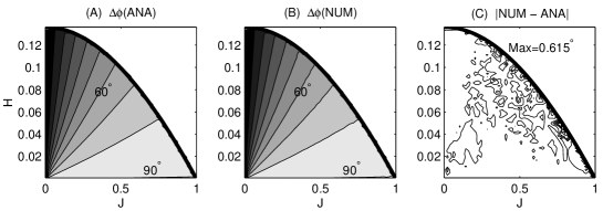
Figure 5: Left-hand panel: precession angle $\Delta\phi$ calculated using the exact analytical formula (57). Center panel: $\Delta\phi$ calculated from numerical integration of the three-wave equations. Note that $\Delta\phi=0$ for $J=0$ and $\Delta\phi=90^{\circ}$ for $H=0$. Right-hand panel: difference in precession angle between the numerical and the analytical solution.

6.1 Determination of the Precession Angle

We now show that the envelope of the motion may be determined to high accuracy by using approximate formulas involving only elementary functions. We use the analytical values as a reference to evaluate the accuracy of the approximate formulas. In Fig. 6 the differences between the exact and approximate expressions for $\Delta\phi$ are shown. The absolute values of these errors are plotted. The maximum error in the DGC formula (Fig. 6(A)) is about $2.2^{\circ}$, and occurs for $J\approx\textstyle\frac{1}{2}$ and $H$ at its maximum permissible value. The error in the alternative formula (72) is of comparable magnitude, with a maximum of about $2.5^{\circ}$ (Fig. 6(B)), but is of opposite sign. The optimal value $\alpha=0.458$ of the parameter in the formula (73) was found by experiment. Fig. 6(C) shows that this formula is significantly more accurate, with a maximum error less than $0.4^{\circ}$. This is a remarkable level of precision, considering the simplicity of the formula. The compensation of errors leads to what might be described as the unreasonable effectiveness of the approximation.

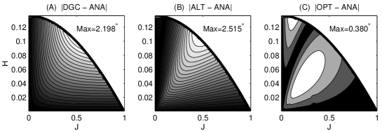
Figure 6: Differences in precession angle $\Delta\phi$ between three approximate formulas and the analytical solution (57). (A) The DGC formula (71); (B) The alternative formula (72); (C) The optimum formula (73). Absolute values are shown. The signs of the errors of (71) and (72) are opposite. The contour interval is $0.1^{\circ}$ in all panels.

6.2 Determination of the Pulsation Amplitude

The extent to which energy is exchanged between the elastic and pendular modes of oscillation may be measured by the relative pulsation amplitude defined as

$$P=\frac{2(C_{2}^{2}-C_{3}^{2})}{N}\,.$$ (74)

This quantity varies from $P=0$ for no energy exchange to $P=1$ for maximal exchange. For $H=0$, it reduces to $P=1-J/N$. Given the invariants $N$, $H$ and $J$, we may compute $P$ by solving the cubic equation $\Phi(Z)=0$ where, as before, $\Phi(Z)=\Phi_{0}(Z)-H^{2}$, with $Z=|C|^{2}$ and $\Phi_{0}$ defined by (26). For determination of the envelope, (74) is ideal. However, for the inverse problem, it must be simplified. Noting that $C_{1}^{2}+C_{2}^{2}+C_{3}^{2}=N$, we may write the pulsation amplitude as

$$P=\frac{2(2C_{2}^{2}+C_{1}^{2}-N)}{N}\,.$$

We have already introduced in (67) a quadratic $\Psi_{0}$ which approximates the cubic $\Phi_{0}$ in the range $[C_{2}^{2},C_{1}^{2}]$. If we use the roots of $\Psi_{0}-H^{2}=0$ as estimates of $C_{1}^{2}$ and $C_{2}^{2}$, an approximate expression for $P$ may be obtained:

$$\framebox{$P=1-\sqrt{\displaystyle{\frac{J^{2}}{N^{2}}+\frac{4H^{2}}{N^{2}Z_{0}}}}\,.$}$$ (75)

For fixed $P$ this represents an ellipse in $(J,H)$-space. The great advantage of (75) is that it can be used to solve the inverse problem. Two special cases follow immediately: when $H=0$ then $P=1-J/N$ (which is exact); when $J=0$ then $P=1-2H/N\sqrt{Z_{0}}$ (which is not exact).

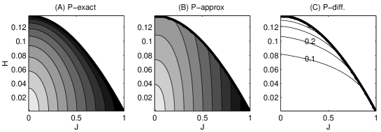
Figure 7: Pulsation amplitude. (A) $P$ based on solving the cubic equation and using (74). (B) $P$ from approximation (75). (C) Magnitude of difference between exact and approximate values The heavy curve is $H_{0}(J)$. The contour interval is $0.1^{\circ}$ in all panels.

We plot the exact values of the pulsation amplitude, obtained by solving the cubic equation $\Phi(Z)=0$, in Fig. 7(A). Note that $P=0$ when $H=H_{0}$ and $P=1$ when $H=J=0$. The approximate values calculated using (75) are shown in Fig. 7(B) and the difference $(P_{\rm approx}-P_{\rm exact})$ in Fig. 7(C). The approximation is quite accurate when $P$ is large. This is the region of primary physical interest, corresponding to strongly pulsating motion. For large values of $H$, the approximation is no longer valid. We have derived several other approximate expressions for $P$, which are more accurate, but also more complicated, than (75).

6.3 Control of the envelope dynamics

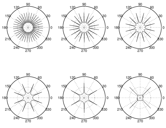
Figure 8: Polar plots of $A_{\rm maj}=|A|+|B|$ against $\phi$, computed from the numerical solution of (9)–(11) for six sets of initial conditions. For all cases, $N=1$ and $P=0.9$, and $J$ and $H$ are computed from (77). Top panels: $\Delta\phi\in\big{\{}10^{\circ},20^{\circ},30^{\circ}\big{\}}$, bottom panels: $\Delta\phi\in\big{\{}45^{\circ},60^{\circ},90^{\circ}\big{\}}$. The integration time in each case corresponds to a total precession of approximately $180^{\circ}$, and both $A_{\rm maj}$ and $-A_{\rm maj}$ are plotted.

The approximate formulas allow us to control the pulsation and precession by a judicious choice of initial conditions. Recall that the precession angle is given, to high accuracy, by (73), which we write

$$\tan\Delta\phi=\frac{J\sqrt{Z_{0}}}{2H}$$ (76)

where $Z_{0}=(N+\alpha J)/2$. This may be used in (75) to eliminate either $H$ or $J$, yielding the two equations

$$P=1-\frac{J}{N}\csc\Delta\phi\qquad\hbox{\rm and}\qquad P=1-\frac{2H}{N\sqrt{Z_{0}}}\sec\Delta\phi\,.$$

But these are instantly invertible, to give equations for $J$ and $H$ in terms of $P$ and $\Delta\phi$:

$$\framebox{$J=N(1-P)\sin\Delta\phi\qquad\hbox{\rm and}\qquad H=\frac{\sqrt{Z_{0}}}{2}N(1-P)\cos\Delta\phi\,.$}$$ (77)

To illustrate the effectiveness of these formulas, six values of the precession angle were chosen: $\Delta\phi\in\big{\{}10^{\circ},20^{\circ},30^{\circ},45^{\circ},60^{\circ},90^{\circ}\big{\}}$. We set $N=1$ and fixed the value of the pulsation amplitude to be $P=0.9$. We then calculated $J$ and $H$ from (77) and computed the numerical solution of the three-wave equations (9)–(11). The initial value of $|C|^{2}$ was taken to be the root $C_{2}^{2}$ of $\Phi(|C|^{2})=0$ having intermediate algebraic magnitude. Then $|A|^{2}$ and $|B|^{2}$ were obtained from the Manley-Rowe relations. The initial phases were all set to zero. Polar plots of $A_{\rm maj}$ against $\phi$ are shown in Fig. 8 (the integration time in each case corresponds to a total precession of about $180^{\circ}$, and both $A_{\rm maj}$ and $-A_{\rm maj}$ are plotted). These plots represent the outer envelope of the horizontal projection of the trajectory of the pendulum bob. It is clear that the precession for the numerical solution is, in each case, close to the value used in (77). We also calculated the pulsation amplitude of the numerical solution and it was, in all cases, within 2% of the prescribed value $P=0.9$. This confirms the effectiveness of the inversion formulas as a means of pre-determining the envelope of the motion.

We note that, in general, the horizontal projection of the trajectory is not a closed curve, but densely covers a region of phase-space. The motion is not periodic but quasi-periodic. The horizontal projection is a closed curve only in the exceptional cases when $\Delta\phi$ and $2\pi$ are commensurate, that is, when their ratio is a rational number. In this case the motion is periodic and the horizontal footprint is a star-like graph, as illustrated in Fig. 8. The number of points in the star is the denominator of the rational number $\Delta\phi/2\pi$ (e.g., $\Delta\phi=80^{\circ}$ yields a nine-pointed star).

7 Conclusion

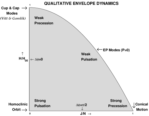
Figure 9: Qualitative features of the envelope dynamics of the swinging spring.

We have presented a complete analytical solution of the three-wave equations, which govern the small-amplitude dynamics of the resonant swinging spring. The periodic variation of the amplitudes is associated with the characteristic pulsation and precession of the system. Several analytical formulas for the precession angle have been presented. We have also derived simplified approximate expressions in terms of elementary functions. The optimal approximation (73) has been shown by numerical experiments to be remarkably accurate, with a maximum error of only $0.4^{\circ}$. The amplitude of the pulsation envelope is determined from the roots of a cubic equation whose coefficients are defined by the invariants. Thus, we have provided a complete and positive answer to Question 1 posed in the Introduction.

The inverse question, Question 2 in §1, has also been answered affirmatively. The approximate formulas (77) give values of $J$ and $H$ which lead to a solution having the prescribed pulsation amplitude and precession angle. They are of high accuracy for strongly pulsating motion, which is the case of primary physical interest.

The qualitative features of the envelope dynamics of the swinging spring are depicted schematically in Fig. 9. The axes are normalized angular momentum $J/N$ and normalized Hamiltonian $H/H_{00}$. The physically accessible domain is shaded. The bounding curve is $H=H_{0}(J,N)$. The pulsation amplitude vanishes on this curve and the solutions are the elliptic-parabolic modes [13]. Regions of the parameter space are indicated where the pulsation amplitude and precession angle take large or small values. The corners of the accessible region represent special solutions. Thus, $(J,H)=(0,H_{00})$ corresponds to the cup-like and cap-like solutions of Vitt and Gorelik [17]. For $(J,H)=(N,0)$, the motion of the spring traces out a cone. Finally $(J,H)=(0,0)$ represents the homoclinic orbit, and includes the case of (unstable) pure vertical oscillations.

Appendix A The Nahm Equations and the Three-wave Equations

The Nahm equations are a set of integrable equations for a three-vector of skew-Hermetian $n\times n$ matrices $(T_{1}(s),T_{2}(s),T_{3}(s))$:

$$\frac{d}{ds}T_{i}=[T_{j},T_{k}]=T_{j}T_{k}-T_{k}T_{j}$$ (78)

where $(i\,j\,k)$ is a cyclic permutation of $(1\,2\,3)$. In the simplest case $s\in(-1,1)$ and the matrices have simple poles as $s\rightarrow\pm 1$.

The Nahm equations were originally discovered because it is possible to use solutions to the equations to construct solutions of the Bogomolny equation [16]. These solutions are called Bogomolny-Prasad-Sommerfield monopoles. The Bogomolny equation occurs as a super-symmetry or minimum energy condition in Yang-Mills Higgs theory and is of interest to theoretical particle physicists.

There is a Lax formulation of the Nahm equations and an associated Lax curve of genus $(n-1)^{2}$. The $n=2$ case is elliptic and the solutions are elliptic functions; in fact, for $n=2$ the Nahm equations reduce to the Euler-Poinsot equations and are easily solved. Surprisingly, it is sometimes also the case that the Nahm equations for $n>2$ can be solved in terms of elliptic functions. This happens when the solution has a symmetry and the quotient of the Lax curve by that symmetry gives a genus-one surface. These symmetries of the Nahm matrices correspond to spatial symmetries of the corresponding monopoles. The group elements act both by conjugation on the Nahm matrices and by rotation of the three-vector of matrices [8, 11].

One example is $n=3$ $D_{2}$ symmetry [10]. The symmetry reduces the Nahm matrices to

$$T_{1} = \frac{i}{\sqrt{2}}\left(\begin{array}[]{ccc}0&F_{1}^{*}&0\\ F_{1}&0&F_{1}\\ 0&F_{1}^{*}&0\end{array}\right),\qquad T_{2}=\frac{1}{\sqrt{2}}\left(\begin{array}[]{ccc}0&F_{2}&0\\ -F_{2}^{*}&0&F_{2}^{*}\\ 0&-F_{2}&0\end{array}\right),$$ (85)

$$T_{3} = \left(\begin{array}[]{ccc}-i\Re\{F_{3}\}&0&-\Im\{F_{3}\}\\ 0&0&0\\ \Im\{F_{3}\}&0&i\Re\{F_{3}\}\end{array}\right),$$ (89)

Substituting these matrices into the Nahm equations gives

$$\frac{dF_{1}}{ds}=F_{2}^{*}F_{3}^{*}$$ (90)

and two others by cyclic permutation. These equations are the ‘explosive interaction’ three-wave equations identified in [2]. They are related to the equations studied in the present paper by $s=it$ with $F_{1}=A^{*}$, $F_{2}=B^{*}$ and $F_{3}=C$.

Appendix B Relationship between Jacobi and Weierstrass forms of the Precession Angle.

To relate the expression (57) obtained by means of Jacobi’s elliptic functions to the expression (48) in terms of the Weierstrass form, we introduce auxiliary constants $d_{+}$ and $d_{-}$ defined by

$$\mathrm{sn}^{2}d_{+}=\gamma_{+}^{2}/k^{2}\,,\qquad\mathrm{sn}^{2}d_{-}=\gamma_{-}^{2}/k^{2}\,.$$

Note that since $\gamma_{\pm}^{2}>k^{2}$, these constants are complex ($d_{+}$ and $d_{-}$ lie on the line between $K$ and $K+iK^{\prime}$). It follows that

$$\mathrm{sn}^{2}d_{+}=\left(\frac{e_{1}-e_{3}}{e_{+}-e_{3}}\right)\,,\quad\mathrm{cn}^{2}d_{+}=-\left(\frac{e_{1}-e_{+}}{e_{+}-e_{3}}\right)\,,\quad\mathrm{dn}^{2}d_{+}=\left(\frac{e_{+}-e_{2}}{e_{+}-e_{3}}\right)\,,$$

with similar expressions involving $d_{-}$. The first of (55) may be written

$$\frac{d\xi}{ds}=-\lambda_{+}-\frac{\lambda_{+}\gamma_{+}^{2}\,\,\mathrm{sn}^{2}s}{1-\gamma_{+}^{2}\,\mathrm{sn}^{2}s}\,,\qquad$$

It may be shown without difficulty, using equation (50), that

$$\lambda_{+}\gamma_{+}^{2}=+ik^{2}\,\mathrm{sn}\,d_{+}\,\mathrm{cn}\,d_{+}\,\mathrm{dn}\,d_{+}\,.$$

Then the solution (56) for $\xi$ may be written

$$\xi-\xi_{0}=-\lambda_{+}s-i\Pi_{1}(s,d_{+},k)\,.$$ (91)

where $\Pi_{1}(s,d_{+},k)$ is another standard form (Jacobi’s form) for the elliptic integral of the third kind ([19], §22.74):

$$\Pi_{1}(s,d_{+},k)=\int_{0}^{s}\frac{k^{2}\,\mathrm{sn}\,d_{+}\,\mathrm{cn}\,d_{+}\,\mathrm{dn}\,d_{+}\,\mathrm{sn}^{2}s}{1-k^{2}\,\mathrm{sn}^{2}d_{+}\,\mathrm{sn}^{2}s}ds\,.$$

The elliptic integral of the second kind is defined (with $x=\mathrm{sn}\,z$) as

$$E(z)\equiv\int_{0}^{z}\mathrm{dn}^{2}z\,dz=\int_{0}^{x}\sqrt{\frac{1-k^{2}x^{2}}{1-x^{2}}}\,dx\,.$$

The complete integral is denoted $E=E(K)$. $E(z)$ is not periodic; the periodic component is represented by Jacobi’s zeta function

$$Z(z)=E(z)-Ez/K\,.$$

This is an odd function with period $2K$. It is related to Jacobi’s theta function, also having period $2K$, by

$$Z(z)=\frac{d}{dz}\log\Theta(z)\,.$$

The elliptic integral of the third kind may now be expressed as follows:

$$\Pi_{1}(z,a,k)=\frac{1}{2}\log\frac{\Theta(z-a)}{\Theta(z+a)}+zZ(a)$$ (92)

For the complete form of the integral, when $z=K$, the logarithmic term vanishes:

$$\Pi_{1}(a,k)=KZ(a)=K\frac{\Theta^{\prime}(a)}{\Theta(a)}\,,$$ (93)

Using this in (91), we obtain the change over a half-period $K$:

$$\textstyle\frac{1}{2}\Delta\xi=-K\lambda_{+}-iKZ(d_{+})\,.$$

Finally, using the analogous expression for $\Delta\eta$, we get the precession angle

$$\framebox{$\Delta\phi=-K(\lambda_{+}-\lambda_{-})-iK\big{(}Z(d_{+})-Z(d_{-})\big{)}$}$$ (94)

This is the change over the period $2K$ (for $s$) or $2K/\nu\sqrt{N}$ (for $t$). The structural similarity between this expression and the result (48) in terms of Weierstrass functions is immediate.

When $J=0$, we have $\lambda_{+}=\lambda_{-}$ and $\gamma_{+}=\gamma_{-}$, so that $d_{+}=d_{-}$ and (94) implies $\Delta\phi=0$. For $H=0$ we have $\lambda_{+}=\lambda_{-}=0$, $d_{+}=K$ and $d_{-}=K+iK^{\prime}$. Then using the relation

$$Z(u+iK^{\prime})=Z(u)-\frac{i\pi}{2K}+\frac{\mathrm{cn}\,u\,\mathrm{dn}\,u}{\mathrm{sn}\,u}$$

with $u=K$, it follows immediately that $\Delta\phi=\pi/2$, in agreement with (49).

Appendix C Approximation Integral with Best Fit at $\mathbf{Z=N_{+}}$.

We approximate $\Phi_{0}=Z(Z-N_{+})(Z-N_{-})$ by a quadratic with a root at $Z-N_{+}$:

$$\Psi_{0}=Z_{0}(Z-N_{+})(Z-Z_{1})$$ (95)

To obtain the best fit at $Z=N_{+}$, we choose $Z_{0}$ and $Z_{1}$ so that

$$\Psi_{0}(Z)-\Phi_{0}(Z)=O\left((Z-N_{+})^{3}\right)\,.$$ (96)

This implies $Z_{0}=N_{+}+J$ and $Z_{1}=N_{+}^{2}/(N_{+}+J)$. Using the software package Maple, it is possible to evaluate the resulting approximate integral

$$\Delta\phi=\frac{HJ}{2}\int^{\infty}_{C_{+}}\frac{d|C|^{2}}{|A|^{2}|B|^{2}\sqrt{\Psi_{0}-H^{2}}}.$$ (97)

where $C_{+}$ is the larger root of $\Psi_{0}-H^{2}=0$. The result is

$$\Delta\phi = \frac{1}{4}\left(2\tan^{-1}{\frac{J(N+J)}{2\sqrt{2}\sqrt{N+3J}H}}+\pi\right)$$ (99)

$$-\frac{H}{4\sqrt{J^{3}-H^{2}}}\left(2\tanh^{-1}\,\frac{J(5J+N)}{2\sqrt{2}\sqrt{J^{3}-H^{2}}\sqrt{N+3J}}+i\pi\right)$$

This gives a rather good approximation: the maximum error is about $1.2^{\circ}$. However, it is not a convenient expression because the factor $\sqrt{J^{3}-H^{2}}$ is sometimes real and sometimes imaginary. Moreover, the expression cannot easily be inverted to give $H$ or $J$ in terms of $\Delta\phi$. In fact, unless $Z_{1}=N_{-}$, any approximating quadratic (95) will give an expression with this problem. Thus, in §5, we choose $Z_{1}=N_{-}$.

References

- [1] M. Abramowitz and I.A. Stegun, Handbook of Mathematical Functions, Dover Publ., New York. 1965.
- [2] M.S. Alber, G.G. Luther, J.E. Marsden and J.M. Robbins, Geometric phases, reduction and Lie-Poisson structure for the resonant three-wave interaction, Physica D 123 (1998), pp. 271–290. http://www.cds.caltech.edu/marsden/bib_src/papers/twi_latex.pdf
- [3] M. Audin, Spinning Tops. A Course on Integrable Systems, Cambridge Univ. Press, Cambridge, 1996.
- [4] P.F. Byrd, P. F. and M. D. Friedman, Handbook of elliptic integrals for engineers and scientists, Second edn. Springer-Verlag, Berlin, 1971.
- [5] H. Dullin, A. Giacobbe and R. Cushman, Monodromy in the resonant swing spring, preprint, 2002. nlin.SI/0212048.
- [6] H.B. Dwight, Tables of integrals and other mathematical data, Macmillan, New York, 1947.
- [7] I.S. Gradshteyn and I.M. Ryzhik, Table of Integrals, Series and Products, Acad. Press, New York. 1965.
- [8] N.J. Hitchin, N.S. Manton and M.K. Murray, Symmetric monopoles, Nonlinearity 8 (1995), p. 661. dg-ga/9503016.
- [9] D.D. Holm and P. Lynch, Stepwise precession of the resonant swinging spring. SIAM J. Appl. Dynam. Sys. 1 (2002), pp. 44–64. nlin.CD/0104038
- [10] C.J. Houghton, Multimonopoles, (Thesis, Cambridge, 1994).
- [11] C.J. Houghton and P.M. Sutcliffe, Tetrahedral and cubic monopoles, Commun. Math. Phys. 180 (1996), p. 342 hep-th/9601146.
- [12] D.F. Lawden, Elliptic functions and applications, Springer-Verlag, New York, 1989.
- [13] P. Lynch, Resonant motions of the three-dimensional elastic pendulum. Intl. J. Nonlin. Mech. 37 (2002), pp. 345–367. http://www.maths.tcd.ie/plynch/Publications/IJNM_Paper.pdf
- [14] P. Lynch, The swinging spring: a simple model for atmospheric balance, in J. Norbury and I. Roulstone (Eds.), Large-scale atmosphere-ocean dynamics: Vol II: geometric methods and models, Cambridge University Press, Cambridge, 2002, pp. 64–108. http://www.maths.tcd.ie/plynch/Publications/AOD_Paper.pdf
- [15] P. Lynch, Resonant Rossby wave triads and the swinging spring. To appear in Bull. Amer. Met. Soc. 84 (2003). http://www.maths.tcd.ie/plynch/Publications/RRTSS.pdf
- [16] W. Nahm, The construction of all selfdual multi-monopoles by the ADHM method, in N.S. Craigie, P. Goddard and W. Nahm, (Eds.), Monopoles in quantum field theory, World Scientific, Singapore, 1982, p. 87.
- [17] A. Vitt and G. Gorelik, Kolebaniya uprugogo mayatnika kak primer kolebaniy dvukh parametricheski svyazannykh linejnykh sistem. Zh. Tekh. Fiz. (J. Tech. Phys.) 3(2-3) (1933), pp. 294–307. Available in English translation: Oscillations of an elastic pendulum as an example of the oscillations of two parametrically coupled linear systems, translated by Lisa Shields, with an introduction by Peter Lynch, Historical Note No. 3, Met Éireann, Dublin (1999). http://www.maths.tcd.ie/plynch/Publications/VandG.pdf
- [18] E.T. Whittaker, A Treatise on the Analytical Dynamics of Particles and Rigid Bodies. 4th Edn. Cambridge Univ. Press, Cambridge 1937.
- [19] E.T. Whittaker and G. N. Watson, A Course of Modern Analysis. 4th Edn. Cambridge Univ. Press, Cambridge 1927.