Uniform semiclassical approximations on a topologically non-
trivial configuration space: The hydrogen atom in an electric field

Abstract

Semiclassical periodic-orbit theory and closed-orbit theory represent a quantum spectrum as a superposition of contributions from individual classical orbits. Close to a bifurcation, these contributions diverge and have to be replaced with a uniform approximation. Its construction requires a normal form that provides a local description of the bifurcation scenario. Usually, the normal form is constructed in flat space. We present an example taken from the hydrogen atom in an electric field where the normal form must be chosen to be defined on a sphere instead of a Euclidean plane. In the example, the necessity to base the normal form on a topologically non-trivial configuration space reveals a subtle interplay between local and global aspects of the phase space structure. We show that a uniform approximation for a bifurcation scenario with non-trivial topology can be constructed using the established uniformization techniques. Semiclassical photo-absorption spectra of the hydrogen atom in an electric field are significantly improved when based on the extended uniform approximations.

1 Introduction

Periodic-orbit theory Gutzwiller90 ; Brack97 and, as a variant for atomic photo-absorption spectra, closed-orbit theory Du88 ; Bogomolny89 have proved to be the most powerful tools available for a semiclassical interpretation of quantum mechanical spectra. Closed-orbit theory provides a semiclassical approximation to the quantum response function

$$g(E)=-\frac{1}{\pi}\sum_{n}\frac{|\left<i|D|n\right>|^{2}}{E-E_{n}+{\rm i}\epsilon}\;,$$ (1)

which involves the energy eigenvalues $E_{n}$ and the dipole matrix elements $\left<i|D|n\right>$ connecting the excited states $n$ to the initial state $i$. Semiclassically, the response function splits into a smooth part and an oscillatory part of the form

$$g^{\rm osc}(E)=\sum_{\rm c.o.}{\cal A}_{\rm c.o.}(E)\,{\rm e}^{{\rm i}S_{\rm c.o.}(E)/\hbar}\;,$$ (2)

where the sum extends over all classical closed orbits starting from the nucleus and returning to it after having been deflected by the external fields. $S_{\rm c.o.}$ is the classical action of the closed orbit. The precise form of the recurrence amplitude $\cal A_{\rm c.o.}$ depends on the geometry of the external field configuration, but it can in any case be calculated from classical properties of the closed orbit. Periodic-orbit theory, which can be applied to any quantum system possessing a classical counterpart, represents the quantum density of states as a sum over the classical periodic orbits in complete analogy with (2).

Both variants of the semiclassical theory share the problem that the semiclassical amplitudes ${\cal A}_{\rm c.o.}$ diverge when the corresponding classical orbits undergo a bifurcation. This failure occurs because close to a bifurcation the classical orbits cannot be regarded as isolated in phase space, as the simple semiclassical expansion (2) assumes. It can be remedied if the individual contributions of the bifurcating orbits to the closed-orbit sum (2) are replaced with a uniform approximation that describes their collective contribution Ozorio87 ; Sieber96 ; Schomerus97b ; Sieber98 . For the generic codimension-one bifurcations of periodic orbits Sieber96 ; Schomerus97b ; Sieber98 as well as closed orbits Bartsch02 ; Bartsch03b , uniform approximations are available in the literature. Typically, bifurcations of higher codimensions are not encountered classically because they split into sequences of codimension-one bifurcations upon an arbitrarily small perturbation. Semiclassically, however, these sequences must be described collectively by a single uniform approximation if the individual bifurcations are sufficiently close Main97a ; Schomerus97a ; Main98a ; Schomerus98 . It can thus be necessary in practice to construct uniform approximations for bifurcation scenarios that are much more complicated than the elementary bifurcations of codimension one.

The crucial step in the derivation of a uniform approximation Sieber98 ; Bartsch02 ; Bartsch03b ; Main97a is the choice of a normal form $\Phi_{a}(x)$ describing the bifurcation scenario. Its stationary points, i.e. the solutions of $\partial\Phi_{a}(x)/\partial x=0$, must be in one-to-one correspondence with the classical closed orbits. In addition, as the parameter $a$ is varied, the stationary points must collide and change from real to complex in accordance with the closed-orbit bifurcations. Once a suitable normal form is known, the uniform approximation assumes the form

$$\Psi(E)=I(a)\,{\rm e}^{{\rm i}S_{0}(E)/\hbar}\;,$$ (3)

where

$$I(a)=\int dx\,p(x)\,{\rm e}^{{\rm i}\Phi_{a}(x)}$$ (4)

and the normal form parameter $a$, the action $S_{0}$ and the unknown function $p(x)$ are determined as functions of the energy $E$ such that the uniform approximation asymptotically reproduces the closed-orbit formula (2) for isolated orbits if the distance from the bifurcation is large.

Usually, the choices of $a$ and $S_{0}$ are unique. By contrast, the asymptotic condition fixes the values of the amplitude function $p(x)$ only at the stationary points of $\Phi_{a}$, so that there remains considerable freedom in its choice. Customarily, a low-order polynomial that interpolates between the given values is chosen. This decision can be justified by observing that a uniform approximation is needed only in the vicinity of the bifurcation, where the stationary points of the normal form are close. Since, in the spirit of the stationary-phase approximation, only the neighbourhood of the stationary points of $\Phi_{a}$ contributes to the integral (4), a Taylor series approximation that is accurate in that region can be expected to be appropriate.

So far, the configuration space of a uniform approximation, i.e. the domain of the normal form variable $x$ and the range of the integral (4) could always be chosen to be a one- or multidimensional Euclidean space. In this paper, we describe an example where this is impossible because for topological reasons the bifurcating orbits cannot be represented as stationary points of a function defined on a Euclidean space. This result is surprising because uniform approximations, as well as the underlying normal forms, are needed to describe closely spaced orbits and bifurcations, and in this sense are local constructions. The topology of the configuration space, on the other hand, reflects its global characteristics. The necessity to base a uniform approximation on a configuration space of a suitable topology thus involves a subtle interplay between local and global aspects of the classical phase space structure. We demonstrate that the established techniques for the construction of uniform approximations are, in principle, applicable to uniform approximations on a topologically non-trivial configuration space, but that additional complications arise when non-local aspects of the dynamics have to be dealt with.

The bifurcation scenario to be discussed arises, e.g., in the hydrogen atom in an electric field. This is an integrable system, and photo-absorption spectra can in principle be obtained by the quantization of classical tori Kon97 ; Kon98 . However, while the torus quantization is restricted to integrable systems, closed-orbit theory is intended to be applicable to arbitrary atomic systems exhibiting either regular, chaotic, or mixed classical behaviour. Therefore, it is of vital interest to see how it can be applied to this apparently simple example. It turns out that to a closed-orbit theory approach the hydrogen atom in an electric field poses the same difficulties in principle as a generic mixed system because the closed orbits undergo plenty of bifurcations. We thus start with a description of the closed orbits in that system in section 2. In section 3 we focus on the bifurcations at low energies and show that in this spectral region a uniform approximation is required that goes beyond the known uniform approximation for the Stark system Gao97 ; Shaw98a ; Shaw98b ; Bartsch02a ; Bartsch03d . This uniform approximation is constructed in section 4, where we also demonstrate that it must rely on a sphere instead of a Euclidean plane as its configuration space. It is compared with the previous uniform approximation, and in section 5 its merits are assessed by the calculation of semiclassical photo-absorption spectra.

2 Closed orbits

The bifurcations of closed orbits in the hydrogen atom in an electric field follow a simple scheme that was described by Gao and Delos Gao94 . Complementary to that work, we demonstrated in a recent publication Bartsch03d that to a large extent the closed orbits and their parameters can be computed analytically. We will now summarize the essential features of the bifurcation scenario. For details, the reader is referred to Bartsch03d .

If we assume the electric field $\vec{F}$ to be directed along the $z$-axis, the Hamiltonian describing the motion of the atomic electron reads, in atomic units,

$$H=\frac{1}{2}\vec{p}^{2}-\frac{1}{r}+Fz\;,$$ (5)

where $r^{2}=x^{2}+y^{2}+z^{2}$. It can be simplified by means of its scaling properties: If the coordinates and momenta are scaled according to $\tilde{\vec{x}}=F^{1/2}\vec{x}$, $\tilde{\vec{p}}=F^{-1/4}\vec{p}$, the classical dynamics is found not to depend on the energy $E$ and the electric field strength $F$ separately, but only on the scaled energy $\tilde{E}=F^{-1/2}E$.

The qualitative simplicity of the bifurcation scenario is due to the well-known fact Born25 ; LandauI that the Hamiltonian (5) is separable in semiparabolic coordinates $\rho_{1}$, $\rho_{2}$, $\varphi$, where

$$\rho_{1}=\sqrt{\tilde{r}-\tilde{z}}\;,\qquad\rho_{2}=\sqrt{\tilde{r}+\tilde{z}}\;,$$ (6)

and $\varphi$ is the azimuth angle around the electric field axis. The angular coordinate $\varphi$ is ignorable, so that its conjugate momentum, the angular momentum $L_{z}$ around the field axis, is conserved. For closed orbits, which pass through the nucleus, $L_{z}=0$. The dynamics of $\rho_{1}$ and $\rho_{2}$ is then given by the equations of motion

$$\begin{split}\rho_{1}^{\prime 2}=\phantom{+}\rho_{1}^{4}+2E\rho_{1}^{2}+c_{1}\;,\\ \rho_{2}^{\prime 2}=-\rho_{2}^{4}+2E\rho_{2}^{2}+c_{2}\;,\\ \end{split}$$ (7)

where $E$ is the energy and the separation constants $c_{1}$ and $c_{2}$ describe the distribution of energy between the $\rho_{1}$ and $\rho_{2}$ degrees of freedom. They are restricted by

$$c_{1}+c_{2}=4\;.$$ (8)

For real orbits the separation constants are constrained to the interval

$$0\leq c_{j}\leq 4\;.$$ (9)

If they fail to meet (9), either $\rho_{1}$ or $\rho_{2}$ assumes complex values, so that a closed “ghost” orbit in the complexified phase space is obtained.

In the simplest cases, one of the $\rho_{j}$ vanishes identically. The electron then moves along the electric field axis. If $c_{1}=0$, the downhill coordinate $\rho_{1}$ is zero. The electron leaves the nucleus in the uphill direction, i.e. in the direction of the electric field, until it is turned around by the joint action of the Coulomb and external fields and returns to the nucleus. After the first return, the uphill orbit is repeated periodically. As the external field provides an arbitrarily high deflecting potential, the uphill orbit is closed at all energies.

The second case of axial motion is obtained if $c_{1}=4$, which corresponds to $\rho_{2}\equiv 0$ and thus to a downhill motion opposite to the direction of the electric field. The downhill orbit closes only if the scaled energy $\tilde{E}$ is less than the scaled saddle point energy $\tilde{E}_{\rm S}=-2$. If $\tilde{E}>\tilde{E}_{\rm S}$, the electron escapes to infinity and the orbit does not close. At scaled energies $\tilde{E}<\tilde{E}_{\rm S}$, the downhill orbit, as the uphill orbit, is repeated periodically.

In general, the motion of the electron will not be directed along the electric field axis and will consist of a superposition of the downhill and uphill motions. In this case a closed orbit is obtained if the downhill and uphill motions close at the same time after $k$ oscillations in the downhill direction and $l$ oscillations in the uphill direction. A closed orbit characterized by integer repetition number $(k,l)$ must satisfy Bartsch03d

$$k\rho_{-}\,{\cal K}(m_{1})=l\rho_{+}\,{\cal K}(m_{2})$$ (10)

with

$$\rho_{+} =\sqrt{-\tilde{E}+\sqrt{\tilde{E}^{2}-c_{1}}}\;,\qquad m_{1} =+\frac{c_{1}}{\rho_{+}^{4}}\;,$$ (11)

$$\rho_{-} =\sqrt{-\tilde{E}+\sqrt{\tilde{E}^{2}+c_{2}}}\;,\qquad m_{2} =-\frac{c_{2}}{\rho_{-}^{4}}$$

and ${\cal K}(m)$ denoting the complete elliptic integral of the first kind Abramowitz .

For given repetition numbers $k,l$ and scaled energy $\tilde{E}$, if we use that $c_{2}=4-c_{1}$ by (8), equation (10) can be solved for the separation parameter $c_{1}$ that specifies the initial conditions of the orbit. A solution only exists if $l>k$. Once $c_{1}$ is known, all orbital parameters relevant to closed-orbit theory can be found analytically. In particular, the classical action of the closed orbit is Bartsch03d

$$S=\frac{2}{3}\,k\rho_{+}^{3}I(m_{1})-\frac{2}{3}\,l\rho_{-}^{3}I(m_{2})$$ (12)

with

$$I(m)=(m-1){\cal K}(m)+(m+1){\cal E}(m)$$ (13)

and the complete elliptic integrals of the first and second kinds ${\cal K}(m)$ and ${\cal E}(m)$ Abramowitz . It is real for both real and ghost orbits.

If the repetition numbers $k$ and $l$ are fixed, for sufficiently low scaled energies $\tilde{E}$ the value of the separation constant $c_{1}$ obtained from (10) is greater than 4, so that the $(k,l)$-orbit is a ghost. As $\tilde{E}$ increases, $c_{1}$ decreases monotonically. At the energy $\tilde{E}_{\rm dest}$ where $c_{1}=4$, the $(k,l)$-orbit becomes real. It is generated (as a real orbit) in a bifurcation off the $k$-th repetition of the downhill orbit, which is characterized by $c_{1}=4$. As $\tilde{E}$ is further increased, the orbit moves away from the downhill orbit and approaches the uphill orbit. At the energy $\tilde{E}_{\rm dest}$ where $c_{1}=0$, the orbit $(k,l)$ collides with the $l$-th repetition of the uphill orbit and is destroyed. At $\tilde{E}>\tilde{E}_{\rm dest}$ the orbit is a ghost again.

The bifurcation energies $\tilde{E}_{\rm gen}$ and $\tilde{E}_{\rm dest}$ can be determined from (10) if $c_{1}=4$ is prescribed for the generation of an orbit, or $c_{1}=0$ for its destruction. For these cases, equation (10) simplifies to

$$\frac{l}{k}=\frac{2^{3/2}}{\pi\sqrt{1+\sqrt{1-\epsilon}}}\,\,{\cal K}\left(\frac{\epsilon}{\left(1+\sqrt{1-\epsilon}\right)^{2}}\right)$$ (14)

in terms of the dimensionless variable $\epsilon=4/\tilde{E}^{2}=(\tilde{E}_{\rm S}/\tilde{E})^{2}$ for the generation of the $(k,l)$ orbit and

$$\frac{k}{l}=\frac{2^{3/2}}{\pi\sqrt{1+\sqrt{1+\epsilon}}}\,\,{\cal K}\left(\frac{-\epsilon}{\left(1+\sqrt{1+\epsilon}\right)^{2}}\right)$$ (15)

for its destruction.

3 Bifurcations at low energies

From the discussion of the closed orbit bifurcations in the preceding section it is evident that there is only a single elementary bifurcation scenario in the hydrogen atom in an electric field, viz. a non-axial orbit being born or destroyed in a collision with an axial orbit. Uniform semiclassical approximations describing this type of bifurcation have been derived by several authors Gao97 ; Shaw98a ; Shaw98b ; Bartsch03d . However, they are only applicable if the individual bifurcations are sufficiently isolated. If they are close, more complicated uniform approximations that provide a collective description of several bifurcations must be found. Thus, there are two spectral regions where the construction of uniform approximations poses a particular challenge:

First, as the Stark saddle energy $\tilde{E}_{\rm S}=-2$ is approached from below, the downhill orbit undergoes infinitely many bifurcations in a finite energy interval before it is destroyed. The periods of the closed orbits created in this way, as the period of the downhill orbit itself, grow arbitrarily large. The actions, however, remain finite, so that the action differences between the orbits stemming from two successive bifurcations become arbitrarily small. Similar cascades of isochronous bifurcations have been found, e.g., in the diamagnetic Kepler problem Wintgen87 and in Hénon-Heiles type potentials Brack01 . Their uniformization remains an open problem. A detailed discussion of this cascade in the Stark system must be referred to future work.

Figure 1: Bifurcations of non-axial orbits off the downhill (+) and uphill ($\times$) orbits in a scaled period vs. scaled energy plot. Bifurcation energies and scaled periods of the bifurcating orbits are indicated. Bifurcations of the downhill orbits only occur below the Stark saddle point energy at $\tilde{E}_{\rm S}=-2$. Dashed lines indicate first, second and third multiples of $\tilde{T}=\frac{2\pi}{3}\sqrt{-2\tilde{E}}$.

Second, non-axial orbits with winding ratios $z=l/k$ close to one are created and destroyed at low energies, and their generation and destruction are closely spaced (see figure 1). Therefore, at low energies a uniform approximation describing both the creation of a non-axial orbit from the downhill orbit and its destruction at the uphill orbit is required. It will be derived in section 4. As a prerequisite, to quantitatively assess its necessity, the asymptotic behaviour of closed-orbit bifurcations at low energies will be investigated in detail in this section.

Bifurcation energies can be determined from equations (14) and (15). As a winding ratio $z=l/k$ close to one corresponds to low bifurcation energies and small values of the parameter $\epsilon=(\tilde{E}_{\rm S}/\tilde{E})^{2}$, approximate bifurcation energies can be obtained by expanding the right hand sides of (14) and (15) in a Taylor series around $\epsilon=0$. We then find the generation and destruction energies

$$\begin{split}\tilde{E}_{\rm gen}&=-\frac{\sqrt{3}}{2\sqrt{z-1}}-\frac{35}{16\sqrt{3}}\,\sqrt{z-1}+{\cal O}\left(z-1\right)^{3/2}\;,\\ \tilde{E}_{\rm dest}&=-\frac{\sqrt{3}}{2\sqrt{z-1}}+\frac{23}{16\sqrt{3}}\,\sqrt{z-1}+{\cal O}\left(z-1\right)^{3/2}\;,\end{split}$$ (16)

for an orbit with a given rational $z$, so that the energy difference

$$\Delta\tilde{E}=\tilde{E}_{\rm dest}-\tilde{E}_{\rm gen}=\frac{29}{8\sqrt{3}}\,\sqrt{z-1}+{\cal O}\left(z-1\right)^{3/2}$$ (17)

indeed vanishes as $z\to 1$.

Figure 2: Schematic illustration of the bifurcation scenario with the definition of the critical quantities. Thick solid line: non-axial real orbit, thick dashed line: non-axial ghost orbit, thin long-dashed line: downhill orbit, thin short-dashed line: uphill orbit. Vertical lines indicate the bifurcation energies.

However, the crucial parameter determining whether or not the bifurcations can be regarded as isolated is not the difference of the bifurcation energies, but rather the action differences between the non-axial orbit and the two axial orbits. For the simple uniform approximation to be applicable, at any energy at least one of the two action differences must be large. In other words (see figure 2), at the critical energy where the actions of the downhill and the uphill orbits are equal, the difference between their action and the action of the non-axial orbit must be large.

To begin with, the actions of the downhill and uphill orbits are given by

$$\begin{split}\tilde{S}_{\begin{array}[]{c}\mbox{\scriptsize{down}}\\[-4.52083pt] \mbox{\scriptsize{up}}\end{array}}=&\sqrt{2}\pi(-\tilde{E})^{-1/2}\pm\frac{3\pi}{4\sqrt{2}}\,(-\tilde{E})^{-5/2}\\ &+\frac{35\pi}{32\sqrt{2}}\,(-\tilde{E})^{-9/2}\pm\frac{1155\pi}{512\sqrt{2}}\,(-\tilde{E})^{-13/2}\\ &+\frac{45045\pi}{8192\sqrt{2}}\,(-\tilde{E})^{-17/2}+{\cal O}(-\tilde{E})^{-19/2}\;.\end{split}$$ (18)

The critical energy for the orbit $(k,l)$ is characterized by the condition $kS_{\rm down}=lS_{\rm up}$, so that $S_{\rm down}/S_{\rm up}=z$. We solve this equation for the critical energy

$$\begin{split}\tilde{E}_{\rm crit}=&-\frac{\sqrt{3}}{2\sqrt{z-1}}-\frac{\sqrt{3}}{8}\,\sqrt{z-1}-\frac{69\sqrt{3}}{64}\,(z-1)^{3/2}\\ &+\frac{209\sqrt{3}}{256}\,(z-1)^{5/2}+{\cal O}(z-1)^{7/2}\;.\end{split}$$ (19)

As expected, the critical energy lies between the two bifurcation energies. If it is substituted into (18), the critical action of the axial orbits

$$\begin{split}\tilde{S}_{\rm ax}=&k\tilde{S}_{\rm down}=l\tilde{S}_{\rm up}\\ =&\frac{2\pi k}{3^{1/4}}\,(z-1)^{1/4}+\frac{3\pi k}{4\cdot 3^{1/4}}\,(z-1)^{5/4}\\ &-\frac{455\pi k}{576\cdot 3^{1/4}}\,(z-1)^{9/4}+{\cal O}(z-1)^{13/4}\end{split}$$ (20)

is obtained.

To determine the critical action of the non-axial orbit, the separation parameter $c_{1}$ for this orbit at the critical energy must be calculated from equation (10), which can be rewritten as

$$\frac{\rho_{-}\,{\cal K}(m_{1})}{\rho_{+}\,{\cal K}(m_{2})}-z=0\;.$$ (21)

Substituting the critical energy (19) into (21), we find

$$\begin{split}&\frac{\rho_{-}\,{\cal K}(m_{1})}{\rho_{+}\,{\cal K}(m_{2})}-z=\frac{29(c_{1}-2)}{24}\,(z-1)^{2}\\ &\qquad+\frac{219\,c_{1}^{2}-876\,c_{1}+526}{144}\,(z-1)^{3}\\ &\qquad+\frac{17951\,c_{1}^{3}-107986\,c_{1}^{2}+188112\,c_{1}-76688}{9216}\,(z-1)^{4}\\ &\qquad+{\cal O}(z-1)^{5}\;.\end{split}$$ (22)

We now make a power series ansatz for $c_{1}$, insert it into (22) and solve for the coefficients to find

$$c_{1}=2+\frac{175}{87}\,(z-1)-\frac{175}{174}\,(z-1)^{2}+{\cal O}(z-1)^{3}\;.$$ (23)

From the knowledge of the critical energy and the separation parameter, the critical action of the non-axial orbit is found to be

$$\begin{split}\tilde{S}_{\rm non}=&\frac{2\pi k}{3^{1/4}}\,(z-1)^{1/4}+\frac{3\pi k}{4\cdot 3^{1/4}}\,(z-1)^{5/4}\\ &-\frac{1151\pi k}{576\cdot 3^{1/4}}\,(z-1)^{9/4}+{\cal O}(z-1)^{13/4}\;.\end{split}$$ (24)

This result agrees with (20) in leading and next-to-leading order. The critical action difference is

$$\Delta\tilde{S}_{\rm crit}=\frac{29\pi q}{24\cdot 3^{1/4}}\,(z-1)^{5/4}+{\cal O}(z-1)^{9/4}$$ (25)

with $q=l-k$. If the critical action difference is written as a function of the critical energy given by (19), it reads

$$\Delta\tilde{S}_{\rm crit}=\frac{29\pi q}{32\sqrt{2}}\,(-\tilde{E}_{\rm crit})^{-5/2}+{\cal O}(-\tilde{E}_{\rm crit})^{-7/2}\;.$$ (26)

Note that due to delicate cancellations occurring during the calculation, all terms of the series expansions given above are needed to obtain the leading-order result (26). Due to these cancellations, the critical action difference is proportional to a high power of the energy, so that it vanishes fast at low energies.

Figure 3: Numerically calculated critical action differences (crosses) for $q=l-k=1$ as a function of the critical energies. The solid line gives the leading-order result (26).

Figure 3 shows numerically computed critical action differences as a function of the pertinent critical energies for $q=1$. The leading-order result (26) is indicated by the solid line. It is accurate even at fairly high energies.

4 Uniform approximation on the sphere

In the hydrogen atom in an electric field, the bifurcation scenarios are largely shaped by the rotational symmetry around the electric field axis: Due to that symmetry, all non-axial orbits occur in one-parameter families, whereas away from a bifurcation the axial orbits are isolated. A normal form describing the bifurcation must also possess a rotational symmetry. Therefore, its configuration space must be at least two-dimensional. It can be chosen to be defined on a Euclidean plane $(x,y)$ and reads Gao97 ; Shaw98a ; Shaw98b ; Bartsch03d

$$\Phi_{a}(x,y)=\frac{1}{4}\,r^{4}-\frac{1}{2}ar^{2}$$ (27)

with a real parameter $a$ and $r^{2}=x^{2}+y^{2}$ the distance from the symmetry centre. Apart from the trivial stationary point at the origin, (27) has a ring of stationary points at $r=\sqrt{a}$, which is real if $a>0$ and imaginary if $a<0$. Thus, (27) describes a family of non-axial real orbits present for $a>0$ which then contracts onto an axial orbit and becomes a family of ghost orbits. It therefore reproduces the elementary bifurcation described in section 2.

In terms of the actions $S_{\rm ax},S_{\rm non}$ and semiclassical amplitudes ${\cal A}_{\rm ax}$, ${\cal A}_{\rm non}$ of the axial and non-axial orbits, respectively, we found the uniform approximation (3) corresponding to the normal form (27) to be Bartsch03d

$$\Psi(E)=\left[\frac{{\cal A}_{\rm non}}{(1+{\rm i})}\,I_{0}+\frac{1}{a}\left(a{\cal A}_{\rm ax}+\frac{1+{\rm i}}{\sqrt{2\pi}}\,{\cal A}_{\rm non}\right)\right]{\rm e}^{{\rm i}S_{\rm ax}}\;,$$ (28)

where

$$a=\pm 2\sqrt{S_{\rm ax}-S_{\rm non}}$$ (29)

and

$$I_{0}={\rm e}^{-{\rm i}a^{2}/4}\left[\frac{1+{\rm i}}{2}-C\left(-\frac{a}{\sqrt{2\pi}}\right)-{\rm i}S\left(-\frac{a}{\sqrt{2\pi}}\right)\right]$$ (30)

with the Fresnel integrals Abramowitz

$$C(x)=\int_{0}^{x}\cos\left(\frac{\pi}{2}\,t^{2}\right)dt\;,\quad S(x)=\int_{0}^{x}\sin\left(\frac{\pi}{2}\,t^{2}\right)dt\;.$$ (31)

We saw in section 3 that it is essential at low energies to construct a uniform approximation capable of simultaneously describing both bifurcations of a non-axial orbit. As the normal form (27) describes only one axial orbit and a non-axial orbit bifurcating out of it, the uniform approximation (28) is unsuitable for this purpose.

A normal form describing both the generation and the destruction of a non-axial orbit must possess two isolated stationary points corresponding to the uphill and downhill orbits and a ring of stationary points related to the family of non-axial orbits. As the normal form parameters are varied, the ring must branch off the first isolated stationary point and later contract onto the second. This is impossible if the normal form is to be defined in a plane, but it is easily achieved if the normal form is based on a sphere. It can then be chosen in such a way that it has isolated stationary points at the poles and a ring of stationary points moving from one pole to the other. A normal form satisfying these requirements is

$$\Phi_{a,b}(\vartheta)=b(\cos\vartheta-a)^{2}\;.$$ (32)

It is given in terms of the polar angle $\vartheta$ on the sphere. Due to the rotational symmetry, it is independent of the azimuth angle $\varphi$, and it contains two real parameters $a$ and $b$ needed to match the two action differences between the three closed orbits.

If, in the vicinity of the poles, $\Phi_{a,b}$ is expanded in terms of the distance $\rho=\sin\vartheta$ from the polar axis, it reads

$$\Phi_{a,b}=b(a-1)^{2}+ba\left(\frac{1}{4}\rho^{4}+\frac{a-1}{a}\rho^{2}\right)+{\cal O}\left(\rho^{6}\right)$$ (33)

around $\vartheta=0$, and

$$\Phi_{a,b}=b(a+1)^{2}-ba\left(\frac{1}{4}\rho^{4}+\frac{a+1}{a}\rho^{2}\right)+{\cal O}\left(\rho^{6}\right)$$ (34)

around $\vartheta=\pi$, so that in both cases (32) reproduces the simpler normal form (27) up to re-scaling. From the coefficients of the quadratic terms in (33) and (34) it is apparent that a ring of stationary points bifurcates off $\vartheta=0$ at $a=1$, and off $\vartheta=\pi$ at $a=-1$.

These conclusions are confirmed by a discussion of the full normal form (32). The ring of stationary points is located at the polar angle $\vartheta_{\rm non}$ satisfying

$$\cos\vartheta_{\rm non}=a\;.$$ (35)

This angle qualitatively corresponds to the starting and returning angle of the non-axial orbit in that it describes its motion from the downhill orbit at $\vartheta=0$ to the uphill orbit at $\vartheta=\pi$. Quantitatively, $\vartheta_{\rm non}$ cannot directly be identified with the classical angle $\vartheta$ because the energy-dependence of the normal form parameters $a$ and $b$ is fixed by matching the action differences rather than the angles. If $-1\leq a\leq 1$, the angle $\vartheta_{\rm non}$ defined by (35) is real. If $a>1$, $\vartheta_{\rm non}$ is purely imaginary, corresponding to a ghost orbit at energies below $\tilde{E}_{\rm gen}$. For $a<-1$, $\vartheta_{\rm non}$ is of the form $\vartheta_{\rm non}=\pi+{\rm i}\alpha$, as is characteristic of a ghost orbit at energies higher than $\tilde{E}_{\rm dest}$.

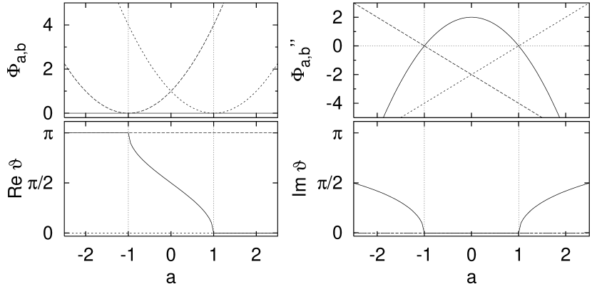
Figure 4: Bifurcation scenario described by the normal form (32) for $b=1$. Location $\vartheta$ of the stationary points, stationary values of the normal form $\Phi_{a,b}$ and stationary values of its second derivative. Solid line: stationary point at $\vartheta_{\rm non}$, long-dashed line: stationary point at $\vartheta=\pi$, short-dashed line: stationary point at $\vartheta=0$.

Figure 5: Orbital parameters for the bifurcations of the (20,21) non-axial orbit. Solid line: non-axial orbit $(20,21)$, long-dashed line: 21st repetition of the uphill orbit, short-dashed line: 20th repetition of the downhill orbit. The vertical lines indicate the bifurcation energies $\tilde{E}_{\rm gen}=-4.155542$ and $\tilde{E}_{\rm dest}=-3.693431$, respectively.

The bifurcation scenario described by the normal form (32) is summarized in figure 4. For $b=1$, the stationary values of (32), the complex polar angles $\vartheta$ where stationary points occur, and the second derivative of $\Phi_{a,b}$ with respect to $\vartheta$ are shown as functions of $a$. Due to the rotational symmetry, the latter is well defined even at the poles.

Figure 4 should be compared to figure 5, which displays the orbital data pertinent to an actual bifurcation scenario. The qualitative agreement between figure 4 and figure 5 is obvious, so that (32) can be seen to describe the bifurcations correctly. (Note that $a$ is a decreasing function of $E$.)

As the normal form (32) has been chosen such as to vanish at the non-axial stationary point $\vartheta_{\rm non}$, the pertinent uniform approximation reads

$$\Psi(E)=I(a,b)\,{\rm e}^{{\rm i}S_{\rm non}(E)}\;,$$ (36)

where $S_{\rm non}(E)$ denotes the action of the non-axial orbit and

$$I(a,b)=\int_{0}^{\pi}d\vartheta\int_{0}^{2\pi}d\varphi\,p(\vartheta)\,{\rm e}^{{\rm i}\Phi_{a,b}(\vartheta)}$$ (37)

with an amplitude function $p(\vartheta)$ to be specified below.

The connection with closed-orbit theory is established with the help of a stationary-phase approximation to the integral (37). If $|a|>1$, the only real stationary points of $\Phi_{a,b}$ are located at the poles, and the asymptotic approximation to (36) reads

$$\begin{split}\Psi(E)\approx&-\frac{\pi{\rm i}}{b(1-a)}\,p(0){\rm e}^{{\rm i}b(1-a)^{2}+{\rm i}S_{\rm non}}\\ &-\frac{\pi{\rm i}}{b(1+a)}\,p(\pi){\rm e}^{{\rm i}b(1+a)^{2}+{\rm i}S_{\rm non}}\;.\end{split}$$ (38)

If $|a|<1$, the contribution

$$\Psi(E)|_{\vartheta_{\rm non}}=2\pi\sqrt{\frac{\pi{\rm i}}{b}}\,p(\vartheta_{\rm non})\,{\rm e}^{{\rm i}S_{\rm non}}$$ (39)

has to be added to (38). These asymptotic expressions should reproduce the simple closed-orbit theory formulae

$${\cal A}_{\rm down}{\rm e}^{{\rm i}S_{\rm down}}+{\cal A}_{\rm up}{\rm e}^{{\rm i}S_{\rm up}}$$ (40)

and

$${\cal A}_{\rm non}{\rm e}^{{\rm i}S_{\rm non}}\;,$$ (41)

respectively. We thus obtain the conditions

$$\begin{split}\Delta S_{\rm down}&=S_{\rm down}-S_{\rm non}=b(1-a)^{2}\;,\\ \Delta S_{\rm up}&=S_{\rm up}-S_{\rm non}=b(1+a)^{2}\;,\end{split}$$ (42)

and

$$\begin{gathered}{\cal A}_{\rm down}=-\frac{\pi{\rm i}}{b(1-a)}\,p(0)\;,\qquad{\cal A}_{\rm up}=-\frac{\pi{\rm i}}{b(1+a)}\,p(\pi)\;,\\ {\cal A}_{\rm non}=2\pi\sqrt{\frac{\pi{\rm i}}{b}}\,p(\vartheta_{\rm non})\end{gathered}$$ (43)

connecting the actions and amplitudes of the downhill, uphill and non-axial orbits to the normal form parameters $a$ and $b$ and to the values of the amplitude function $p(\vartheta)$.

Equation (42) can be solved for the normal form parameters to yield

$$a=\frac{\sqrt{\Delta S_{\rm up}}\mp\sqrt{\Delta S_{\rm down}}}{\sqrt{\Delta S_{\rm up}}\pm\sqrt{\Delta S_{\rm down}}}$$ (44)

and

$$b=\frac{\Delta S_{\rm down}}{(1-a)^{2}}=\frac{\Delta S_{\rm up}}{(1+a)^{2}}\;,$$ (45)

where the upper or lower sign has to be chosen if the non-axial orbit is real or complex, respectively.

If we set $p(\vartheta)$ equal to a constant in (43), we obtain the constraints

$$\begin{split}\frac{1+{\rm i}}{2}\,\sqrt{\frac{b}{2\pi}}\,{\cal A}_{\rm non}&=-b(1-a)\,{\cal A}_{\rm down}\\ \frac{1+{\rm i}}{2}\,\sqrt{\frac{b}{2\pi}}\,{\cal A}_{\rm non}&=-b(1+a)\,{\cal A}_{\rm up}\end{split}$$ (46)

the amplitudes must satisfy close to the individual bifurcations. Numerically, (46) can be verified to hold in the neighbourhood of the bifurcations.

To obtain a complete uniform approximation, we make the ansatz

$$p(\vartheta)=p_{0}+p_{1}(\cos\vartheta-a)+p_{2}(\cos\vartheta-a)^{2}$$ (47)

for the amplitude function. The coefficients are given by

$$\begin{gathered}p_{0}=p(\vartheta_{\rm non})\;,\\ p_{1}=\frac{(1+a)^{2}p(0)-4a\,p(\vartheta_{\rm non})-(1-a)^{2}p(\pi)}{2(1-a^{2})}\;,\\ p_{2}=\frac{(1+a)p(0)-2p(\vartheta_{\rm non})+(1-a)p(\pi)}{2(1-a^{2})}\end{gathered}$$ (48)

with the values $p(0)$, $p(\pi)$ and $p(\vartheta_{\rm non})$ determined from (43). Due to (46), all coefficients are finite everywhere.

With this choice, the uniform approximation (36) reads

$$\Psi(E)=p_{0}I_{0}+p_{1}I_{1}+p_{2}I_{2}$$ (49)

with the integrals

$$\begin{split}I_{0}&=\int_{0}^{2\pi}d\varphi\int_{0}^{\pi}d\vartheta\sin\vartheta\,{\rm e}^{{\rm i}b(\cos\vartheta-a)^{2}}\\ &=2\pi\sqrt{\frac{\pi}{2b}}\left(C\left(\sqrt{\frac{2b}{\pi}}(1-a)\right)+{\rm i}S\left(\sqrt{\frac{2b}{\pi}}(1-a)\right)\right.\\ &\phantom{=2\pi\sqrt{\frac{\pi}{2b}}\,}\left.+\,C\left(\sqrt{\frac{2b}{\pi}}(1+a)\right)+{\rm i}S\left(\sqrt{\frac{2b}{\pi}}(1+a)\right)\right)\end{split}$$ (50)

in terms of the Fresnel integrals (31),

$$\begin{split}I_{1}&=\int_{0}^{2\pi}d\varphi\int_{0}^{\pi}d\vartheta\sin\vartheta\,(\cos\vartheta-a)\,{\rm e}^{{\rm i}b(\cos\vartheta-a)^{2}}\\ &=\frac{\pi{\rm i}}{b}\left({\rm e}^{{\rm i}b(1+a)^{2}}-{\rm e}^{{\rm i}b(1-a)^{2}}\right)\end{split}$$ (51)

and

$$\begin{split}I_{2}&=\int_{0}^{2\pi}d\varphi\int_{0}^{\pi}d\vartheta\sin\vartheta\,(\cos\vartheta-a)^{2}\,{\rm e}^{{\rm i}b(\cos\vartheta-a)^{2}}\\ &=-{\rm i}\frac{d}{db}I_{0}\\ &=-\frac{\pi{\rm i}}{b}\left((1-a)\,{\rm e}^{{\rm i}b(1-a)^{2}}+(1+a)\,{\rm e}^{{\rm i}b(1+a)^{2}}\right)+\frac{{\rm i}}{2b}I_{0}\;.\end{split}$$ (52)

All integrals are finite as they stand, they do not require any regularization. This somewhat atypical behaviour can be traced back to the fact that the domain of integration in this case is compact.

Figure 6: Uniform approximation for the generation and destruction of the (20,21) non-axial orbit for the electric field strengths (a) $F=10^{-2}$, (b) $F=10^{-6}$, (c) $F=10^{-10}$. Solid lines: Uniform approximation (49), long-dashed lines: uniform approximation (28) for isolated bifurcations, short-dashed lines: isolated-orbits approximation.

As an example, figure 6 compares the uniform approximation (49) for the orbit (20,21) and three different electric field strengths to the isolated-orbits approximation and to the uniform approximation (28) for isolated bifurcations. For the latter, the non-axial orbit and the axial orbit for which the action difference is smaller are combined into the uniform approximation, whereas the second axial orbit is treated as isolated.

For the high electric field strength $F=10^{-2}$ in figure 6(a), in the energy range shown none of the uniform approximations reaches the asymptotic region where they agree with the isolated-orbits approximation on either side of the bifurcations. Between the two bifurcations, the isolated-bifurcations approximation appears just to arrive at its asymptotic behaviour before the second bifurcation is felt. The behaviour of the uniform approximation on the sphere is completely different there.

If the field strength is decreased, both uniform approximations reach their asymptotic regions faster. For $F=10^{-6}$, they approach the isolated-orbits approximation at roughly equal pace on both sides of the bifurcations. Between the bifurcations, the isolated-bifurcations approximation now clearly attains its asymptotic behaviour, whereas the uniform approximation on the sphere exhibits qualitatively similar behaviour, but differs significantly from the other two in quantitative terms. It requires the even lower field strength of $F=10^{-10}$ used in figure 6(c) until both uniform approximations agree with the isolated-orbits result in the region between the bifurcations.

The uniform approximation on the sphere was constructed because in the energy region between the bifurcations the isolated-bifurcations approximation must fail for low energies and high field strengths. However, it turns out to reach its asymptotic agreement with the isolated-orbits results considerably more slowly than the isolated-bifurcations approximation. In cases where the latter reproduces the isolated-orbits results between the bifurcations, of course, no further uniformization is required.

5 Semiclassical Stark spectra

More information on the virtue of the uniform approximation on the sphere can be obtained from a calculation of actual semiclassical spectra. To this end we calculated semiclassical photo-absorption spectra for the hydrogen atom in an electric field based on closed-orbit theory and including uniform approximations. To low-resolution, a semiclassical spectrum can be obtained if the contributions of orbits up to a maximum period $\widetilde{T}_{\rm max}$ are included in the closed-orbit sum (2).

We will present results for the photoexcitation of the $1s$ ground state of the hydrogen atom in an electric field of strength $F=10^{-8}\,{\rm a.u.}\hat{=}51.4\,{\rm V/cm}$. The exciting photon is assumed to be linearly polarized along the field axis. In the closed-orbit summation, the uniform approximation (49) based on the sphere will be used if the action differences between a non-axial orbit and both the downhill and uphill orbits it bifurcates out of are smaller than $2\pi$. In the other cases, we revert to the simple uniform approximation (28) or the isolated-orbits approximation, as appropriate.

Figure 7: Low-resolution photo-absorption spectrum: (a) semiclassical spectrum not using and (b) using the uniform approximation on the sphere, (c) smoothed quantum spectrum. The scaled cut-off time is $\widetilde{T}_{\rm max}=30$.

Figure 7 shows a comparison between the semiclassical spectra obtained from the simple uniform approximation only (figure 7(a)), the closed-orbit summation with the uniform approximation based on the sphere (figure 7(b)), and an appropriately smoothed quantum spectrum (figure 7(c)). Note that only the oscillatory part of the semiclassical spectra is plotted, so that the base line is slightly shifted away from zero. This shift is absent in the quantum spectrum.

It has already been found in Bartsch03d that, if only the simple uniform approximation (3) is used, the spectral lines close to the centres of the $n$-manifolds tend to have considerable strengths although they are negligibly weak in the quantum spectrum. If the uniform approximation on the sphere is used, on the one hand the line strengths develop a second maximum at the centre of a manifold. On the other hand, however, the absolute intensity of the central lines is considerably reduced, so that the overall intensity distribution within an $n$-manifold is reproduced much better than with the isolated-bifurcations approximation only.

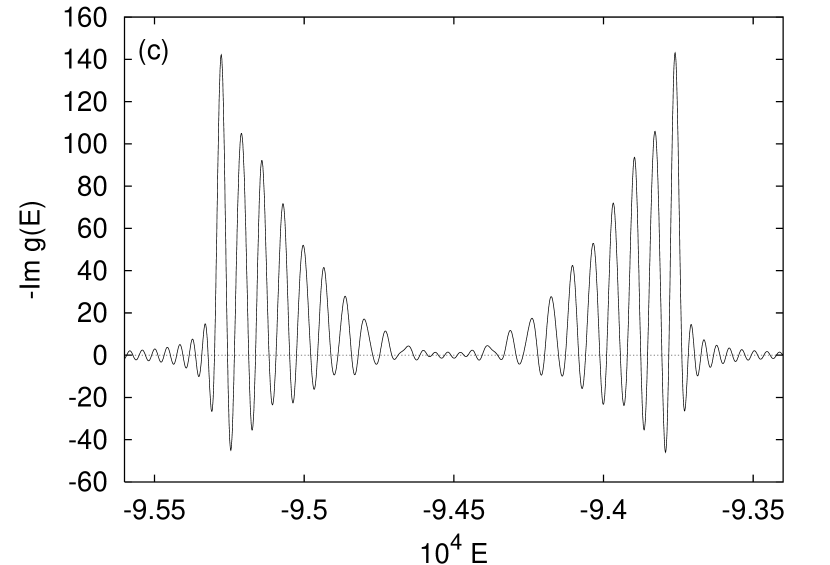
Figure 8: The manifold $n=23$ from the spectra shown in figure 7. (a) Semiclassical spectrum not using and (b) using the uniform approximation on the sphere, (c) smoothed quantum spectrum.

These observations can be confirmed if one of the $n$-manifolds is viewed in more detail. Figure 8 compares the low-resolution semiclassical spectra of the manifold $n=23$, which is the lowest $n$-manifold included in the calculation, to the quantum spectrum. In the spectrum shown in figure 8(a), which uses the simple uniform approximation (28) only, the lines at the edges of the manifold are the strongest, and the line strengths decrease gently toward the centre. The line shapes are slightly asymmetric, although the asymmetry is weaker than at higher energies Bartsch03d . In the spectrum obtained using the uniform approximation on the sphere (figure 8(b)), the strong outer lines of the manifold are virtually identical to those in the previous spectrum, but the central lines are distorted. On the other hand, again, as the central lines are weaker in the spectrum of figure 8(b) than in figure 8(a), the distribution of intensities within the manifold is described more accurately if the uniform approximation on the sphere is used.

In addition to the calculation of low-resolution semiclassical spectra, we can use the techniques of Bartsch02a ; Bartsch03d to compute individual spectral lines. The results do not depend strongly on the choice of the uniform approximations; the high-resolution spectra obtained from the spectrum in figure 7(b) which use the uniform approximation on the sphere (see Bartsch02 ) are virtually identical to those presented in Bartsch03d that apply the simple uniform approximation (figure 7(a)) only.

The uniform approximation on the sphere, although it satisfies the correct asymptotic conditions and is well adapted to the bifurcation scenario qualitatively, in quantitative terms does not yield absolutely precise results. The problem is probably connected to the non-trivial spherical topology of the configuration space of the uniform approximation: The construction of uniform approximations of the type (3) relies on the assumption that the unknown phase function in the diffraction integral can be mapped to a certain standard form by a suitable coordinate transformation. The fundamental theorems of catastrophe theory Castrigiano93 ; Poston78 guarantee that this is possible locally. In a Cartesian configuration space and close to a bifurcation, all stationary points of the normal form are close to the origin, so that coordinate regions away from the origin can, in the spirit of the stationary-phase approximation, be assumed not to contribute to the diffraction integral. A local mapping of the function in the exponent to the normal form and a local approximation to the amplitude function by means of a Taylor series thus suffice to obtain good results. By contrast, on the spherical configuration space a global approximation to the unknown functions must be sought because the stationary points are distributed across the sphere: There is a stationary point at each pole. In the case at hand, we tried replacing the $(\cos\vartheta-a)^{2}$-term in the amplitude function (47) with $\sin\vartheta$, which also gives a rough approximation to the actual amplitude function. The alteration has no significant effect on the result. The construction of a quantitatively more reliable uniform approximation will presumably require a deeper global understanding of the bifurcation scenarios. It remains a worthwhile challenge for future research to devise an easy-to-apply technique for the construction of uniform approximations that takes full account of the classical phase space topology.

6 Conclusion

We have discussed the bifurcations of closed orbits in the hydrogen atom in an electric field. At low scaled energies a uniform semiclassical approximation is required that simultaneously describes both the generation and the destruction of a non-axial orbit. Its construction was carried out. Beyond its significance to the Stark system, it is of interest for reasons of principle because it uses a sphere instead of a Euclidean plane as its configuration space and thus is the first uniform approximation introduced in the literature that relies on a topologically non-trivial configuration space. It could be demonstrated that uniform approximations with a non-Euclidean configuration space can indeed be constructed and allow for the semiclassical calculation of significantly improved photo-absorption spectra of the hydrogen atom in an electric field.

References

- (1) M. C. Gutzwiller, Chaos in Classical and Quantum Mechanics, Springer-Verlag, New York, 1990.
- (2) M. Brack and R. K. Bhaduri, Semiclassical Physics, Addison-Wesley Publishing Company, Reading, Mass., 1997.
- (3) M. L. Du and J. B. Delos, Phys. Rev. A 38, 1896 and 1913 (1988).
- (4) E. B. Bogomolny, Sov. Phys. JETP 69, 275 (1989).
- (5) A. M. Ozorio de Almeida and J. H. Hannay, J. Phys. A 20, 5873 (1987).
- (6) M. Sieber, J. Phys. A 29, 4715 (1996).
- (7) H. Schomerus and M. Sieber, J. Phys. A 30, 4537 (1997).
- (8) M. Sieber and H. Schomerus, J. Phys. A 31, 165 (1998).
- (9) T. Bartsch, The hydrogen atom in an electric field and in crossed electric and magnetic fields: Closed-orbit theory and semiclassical quantization., Cuvillier, Göttingen, Germany, 2002.
- (10) T. Bartsch, J. Main, and G. Wunner, Phys. Rev. A, submitted. LANL preprint nlin.CD/0212017.
- (11) J. Main and G. Wunner, Phys. Rev. A 55, 1743 (1997).
- (12) H. Schomerus, Europhys. Lett. 38, 423 (1997).
- (13) J. Main and G. Wunner, Phys. Rev. E 57, 7325 (1998).
- (14) H. Schomerus, J. Phys. A 31, 4167 (1998).
- (15) V. Kondratovich and J. B. Delos, Phys. Rev. A 56, R5 (1997).
- (16) V. Kondratovich and J. B. Delos, Phys. Rev. A 57, 4654 (1998).
- (17) J. Gao and J. B. Delos, Phys. Rev. A 56, 356 (1997).
- (18) J. A. Shaw and F. Robicheaux, Phys. Rev. A 58, 1910 (1998).
- (19) J. A. Shaw and F. Robicheaux, Phys. Rev. A 58, 3561 (1998).
- (20) T. Bartsch, J. Main, and G. Wunner, Phys. Rev. A 66, 033404 (2002).
- (21) T. Bartsch, J. Main, and G. Wunner, J. Phys. B, submitted. LANL preprint nlin.CD/0212046.
- (22) J. Gao and J. B. Delos, Phys. Rev. A 49, 869 (1994).
- (23) M. Born, Vorlesungen über Atommechanik, Springer, Berlin, 1925.
- (24) L. D. Landau and E. M. Lifshitz, Mechanics, Pergamon Press, Oxford, 1960.
- (25) M. Abramowitz and I. A. Stegun, Pocketbook of Mathematical Functions, Verlag Harri Deutsch, Frankfurt/Main, 1984.
- (26) D. Wintgen, J. Phys. B 20, L511 (1987).
- (27) M. Brack, Found. Phys. 31, 209 (2001).
- (28) D. P. L. Castrigiano and S. A. Hayes, Catastrophe Theory, Addison-Wesley Publishing Company, Reading, MA, 1993.
- (29) T. Poston and I. Stewart, Catastrophe Theory and its Applications, Pitman, Boston, 1978.