Recovering Isotropic Statistics in Turbulence Simulations: The Kolmogorov 4/5th-Law

Abstract

One of the main benchmarks in direct numerical simulations of three-dimensional turbulence is the Kolmogorov 1941 prediction for third-order structure functions with homogeneous and isotropic statistics in the infinite-Reynolds number limit. Previous DNS techniques to obtain isotropic statistics have relied on time-averaging structure functions in a few directions over many eddy turnover times, using forcing schemes carefully constructed to generate isotropic data. Motivated by recent theoretical work which removes isotropy requirements by spherically averaging structure functions over all directions, we will present results which supplement long-time averaging by angle-averaging over up to 73 directions from a single flow snapshot. The directions are among those natural to a square computational grid, and are weighted to approximate the spherical average. The averaging process is cheap, and for the Kolmogorov 1941 4/5ths law, reasonable results can be obtained from a single snapshot of data. This procedure may be used to investigate the isotropic statistics of any quantity of interest.

I Introduction

Both experimental and numerical studies of turbulence have attempted to observe the 1941 predictions of A.N. Kolmogorov K41b for the statistics of isotropic, homogeneous, fully developed turbulence in the limit of infinite Reynolds number in an incompressible fluid. A main result of the theory is the so-called “4/5-law”

$$\langle(\delta u_{L}({\bf r},{\bf x}))^{3}\rangle = -\frac{4}{5}\varepsilon r$$ (1)

$$\delta u_{L}({\bf r},{\bf x}) = [{\bf u}({\bf x}+{\bf r})-{\bf u}({\bf x})]\cdot\hat{\bf r}$$

$$\hat{\bf r} = {\bf r}/r$$

where $\langle\cdot\rangle$ denotes ensemble averaging. The lefthand side of Eq. 1 is the well-known third-order longitudinal structure function. The length scale $r$ must lie in the inertial range $\eta<<r<<L$, sufficiently far from the large scales $L$ and the dissipation scales given by the Kolmogorov length $\eta$. The mean energy dissipation rate of the flow is given by $\varepsilon$. The 4/5ths law is one of the few exact, non-trivial results known in the theory of statistical hydrodynamics. It may be reformulated in terms of other components of the structure function by using the incompressibility constraint MYII

$$\langle\delta u_{L}(\delta u_{T})^{2}\rangle=\frac{1}{6}\frac{\partial}{\partial r}(r\langle(\delta u_{L})^{3}\rangle)$$ (2)

where $\delta u_{T}$ is a velocity increment along a vector transverse to the separation vector ${\bf r}$. In Eq. 2 and henceforward, the vector argument ${\bf r}$ is implicit. This combined with the Eq.1 gives “4/15ths law” and the “4/3rds law”

$$\langle\delta u_{L}(\delta u_{T})^{2}\rangle=-\frac{4}{15}\varepsilon r$$ (3)

$$\langle\delta u_{L}|\delta{\bf u}|^{2}\rangle=-\frac{4}{3}\varepsilon r$$ (4)

where $|\delta{\bf u}|$ denotes the total magnitude of the velocity difference across ${\bf r}$. We will refer to the three laws given by Eqs. (1), (3) and (4), and the related theory collectively as K$41^{3}$.

The K$41^{3}$ results have served as invaluable benchmarks for the empirical study of high-Reynolds number turbulence in both experiments and numerical simulations. Considered as exact results, they have allowed investigators to assess the degree to which homogeneous, isotropic, and high Reynolds number conditions have been attained. Furthermore, the derivation of the K$41^{3}$ relations requires a fundamental, unproven assumption, namely, that turbulent energy dissipation has a strictly positive limit as viscosity tends to zero. Hence, the validity of the K$41^{3}$ relations constitute an important test of this basic assumption. Experiments in high-Reynolds number turbulence performed over the past half-century do, by and large, support the linear scaling in $r$ of the third-order structure functions. The convergence to the 4/5ths coefficient is quite slow as Reynolds number increases for large scale anisotropic experiments SVBSCC96 ; BD01 , although there is empirical consensus that indeed this is asymptotically the correct coefficient. Recent numerical simulations GFN02 of isotropically forced Navier-Stokes also emphasize the slow approach to the 4/5ths law as the Reynolds numbers are pushed as high as computational power would allow. A key feature of both experimental and numerical endeavors, is the large volumes of data required – very long time-averages, extending over many integral length-scales or eddy-turnover times are needed to obtain adequate statistics and to observe the trend toward K$41^{3}$.

A modified version of the 4/5ths law, which does not assume isotropy of the flow, now exists. Nie and Tanveer NieTan99 proved that the 4/3rds and consequently, the 4/5ths laws can be recovered in homogeneous, but not necessarily isotropic flows,

$$\langle(\delta u_{L})^{3}\rangle = \lim_{T\rightarrow\infty}\frac{1}{T}\int^{T}_{0}dt\int\frac{d\Omega}{4\pi}\int\frac{d{\bf x}}{L^{3}}[\delta u_{L}({\bf r};{\bf x},t)]^{3}$$ (5)

$$= -\frac{4}{5}\varepsilon r.$$

The angle integration $d\Omega$ integrates in ${\bf r}$ over the sphere of radius $r$. For each point ${\bf x}$ the vector increment ${\bf r}$ is allowed to vary over all angles and the resulting longitudinal moments are integrated. The integration over ${\bf x}$ is over the entire flow domain. The integration over time $t$ extends over long-times, and the long time average is consistent with the ensemble average of the original K41 theory since ergodicity allows identification of ensemble-averages with time-averages Frisch95 . In Eq. 5, the integration over $\Omega$ extracts the isotropic component of a generally anisotropic flow. This is fully consistent with recent experimental ADKLPS98 ; KLPS00 and numerical ABMP99 ; BLMT02 efforts to quantify anisotropic contributions by projecting the structure function onto a particular irreducible representation, labeled by $j=0,1,\dots$, of the SO(3) symmetry group. The angle-averaged Eq. 5 correspond to projecting onto the $j=0$ (isotropic) sector by integration over the sphere. The authors of NieTan99 do not perform numerically the average over the sphere. However, they do point out that the direction of ${\bf r}$ matters strongly. In their anisotropic DNS simulation at moderate Reynolds number, the result of taking ${\bf r}$ along a coordinate direction gave very poor agreement with the laws, whereas taking ${\bf r}$ along a body-diagonal as defined by the square-grid gave much better agreement.

A local version of the 4/3rds law was recently derived by J. Duchon and R. Robert DucRob99 . Subsequently, G.L. Eyink Eyink02 derived the corresponding version of the 4/5ths and 4/15ths laws. The statement is the following: Given $any$ local region $B$ of size $R$ of the flow, for $r<<R$, and in the limits $\nu\rightarrow 0$, next $r\rightarrow 0$, and finally $\delta\rightarrow 0$,

$$\langle(\delta u_{L})^{3}\rangle_{(\Omega,B)} = \lim_{\delta\rightarrow 0}\frac{1}{\delta}\int^{t+\delta}_{t}d\tau\int\frac{d\Omega}{4\pi}\int_{B}\frac{d{\bf x}}{R^{3}}[\delta u_{L}({\bf r};{\bf x},\tau)]^{3}$$ (6)

$$= -\frac{4}{5}\varepsilon_{B}r.$$

for almost every (Lebesgue) point $t$ in time, where $\varepsilon_{B}$ is the instantaneous mean energy dissipation rate over the local region $B$. This version of the K$41^{3}$ results does not require isotropy or homogeneity of the flow. Long-time or ensemble averages are also not required as in the original K41 theory Frisch95 . The Duchon-Robert DucRob99 and Eyink Eyink02 versions of K$41^{3}$ are truly local in space and time.

We are motivated in the present work by the existence of isotropic statistics embedded in anisotropic data as suggested by previous work. It is clear that both experiments and simulations face intrinsic difficulties in achieving the high-Reynolds numbers and isotropic limit required by K41 theory. Both anisotropy and finite Reynolds numbers conspire to shorten the inertial range. Experiments have achieved Reynolds numbers several orders of magnitude higher than simulations. The indication is that at such high Reynolds numbers, the large scale anisotropies decay faster than the isotropic scales, allowing the latter to dominate at small scales KurSre00 . However, while the linear scaling in $r$ of the third-order structure function is fairly robust, the coefficient exhibits only a slow trend toward 4/5 as indicated by the numerical work of GFN02 . It is clear that for anisotropic forcing, some choices of directions for the vector increment ${\bf r}$ are more “isotropic” than others NieTan99 .

The concept of averaging over the sphere in order to extract the isotropic component of turbulence data has existed for some time ALP99 ; KSreview . Present high-Reynolds number experiments provide limited data – often only a few spatial points of data acquisition, with vector increment directions limited by the location of the probes and the implementation of a suitable space-time surrogation (Taylor’s hypothesis). Such configurations are not suitable to spherical averaging. Numerical data has, in principle, complete space-time information of the flow. However, the interpolation of square grid data over spherical shells has been deemed too expensive NieTan99 , or, when some such interpolation scheme is implemented, has not been used at sufficiently high Reynolds numbers as will allow for observations of the K41 type ABMP99 . The new angle-averaged and “local” laws of NieTan99 ; DucRob99 ; Eyink02 provide us with the theoretical impetus to investigate and extract the isotropic component of the flow in high-Reynolds number anisotropic turbulence. We use a novel means of taking the average over angles which avoids the expense and effort of interpolating the square-grid data over spherical shells.

In section II we discuss the numerical method and describe the stochastic and deterministic numerical forcing schemes used in the past and reimplemented by us. In section III we present an easily implemented scheme to average over a finite number of angles. Using the second and third-order isotropy relations, we demonstrate that this scheme is a good approximation to the true spherical average. We then present results for the angle-averaged third-order structure functions computed both from a snapshot of the flow at a single instant in time, and from time-averaging the data from several snapshots. A summary and concluding discussion of the results is given in section IV.

II Numerical Simulations

The numerical simulation of the forced Navier-Stokes equation for an incompressible flow are given by

$$\partial_{t}{\bf u}+{{\bf\omega}\times{\bf u}}+\nabla\phi = \nu\nabla^{2}{\bf u}+{\bf f}$$ (7)

$$\nabla\cdot{\bf u} = 0$$ (8)

where the vorticity $\omega=\nabla\times{\bf u}$ and $\phi$ is determined so as to maintain $\nabla\cdot{\bf u}=0$. The domain is a periodic box of side $L=2\pi$ with $N=512$ grid points to a side. A standard Fourier pseudo-spectral method is used for the spatial discretization and the equations are integrated in time using a fourth-order Runge-Kutta scheme. Aliasing errors from the nonlinear term are effectively controlled by removing all coefficients with wave-number magnitude greater than $k_{max}=\frac{\sqrt{2}}{3}N$. The code is optimized for distributed memory parallel computers and uses MPI for inter-process communication. The runs were made using 256 processors of a Compaq ES45 cluster.

We make use of two different types of low wave number forcing. The first is modeled after the deterministic forcing schemes described in Kerr94 ; SVBSCC96 ; OvePop98 , where the energy in a few low wave numbers is relaxed back to a target spectrum. We refer to the output using this forcing as the deterministic dataset. The second forcing is the stochastic forcing used in GFN02 , where the Fourier coefficients of ${\bf f}$ are chosen randomly, and we refer to the data produces with this forcing as the stochastic dataset. Both forcings have advantages and disadvantages. The deterministic forcing equilibrates quickly and has less variance in time so that less data is needed for converged time averages. But there is an unavoidable anisotropy throughout the simulation if the forcing is restricted to the lowest wave numbers. The stochastic forcing has a larger variance in time so that data from more snapshots is needed to obtain converged time averages, but statistics from those snapshots are observed to be more isotropic. We perform both kinds of forcing in order to demonstrate the equivalence of the results when angle-averaging is applied to the data.

Parameters of interest for both simulations are given in Table 1. For the stochastic forcing, we have chosen parameters similar to those used for the $512^{3}$ simulations in GFN02 . The parameters for the deterministic case were chosen so that $R_{\lambda}$ would be similar in both cases.

Data set	$N$	$\nu$	$\varepsilon$	$k_{max}\eta$	$R_{\lambda}$	$n_{s}$	$n_{r}$
Stochastic	512	$6\times 10^{-4}$	.5	1.1	263	6	6
Deterministic	512	$4\times 10^{-3}$	156	1.1	249	1	6

Table 1: The parameter values for the two data sets. N = Number of grid points per coordinate direction; $\nu$ = viscosity; $\varepsilon$ = Mean energy dissipation rate $\eta$ = Kolmogorov scale; $R_{\lambda}$ = Taylor microscale Reynolds number; $n_{s}$ = number of eddy turnover times to spin up; $n_{r}$ = number of eddy turnover times computed after spin up.

II.1 Deterministic forcing

We first define the energy in each spherical wave number $k$ in the usual way:

$$E(k)=\sum_{k-.5\leq|{\bf k}|<k+.5}\frac{1}{2}|\tilde{\bf u}_{\bf k}|^{2}$$ (9)

where $\tilde{\bf u}_{\bf k}$ is the $k$th Fourier coefficient of ${\bf u}$. We then choose a target spectrum function given by $F(k)$, which we set to $F(1)=F(2)=.5$ and $F(k)=0$ for $k>2$. We generate a velocity field $\tilde{\bf v}_{\bf k}$ with energy $F(k)$ by setting

$$\tilde{\bf v}_{\bf k}=\sqrt{\frac{F(k)}{E(k)}}\,\tilde{\bf u}_{\bf k}$$

The Fourier coefficients of the forcing function are then given by

$$\tilde{\bf f}_{\bf k}=\left\{\begin{array}[]{ll}\tau\left(\tilde{\bf v}_{\bf k}-\tilde{\bf u}_{\bf k}\right),&\qquad F(k)>E(k)\\ 0,&\qquad F(k)\leq E(k)\end{array}\right.$$

The relaxation parameter is chosen as $\tau^{-1}=2|\nabla u|$, a simplified version of the formula given in OvePop98 .

This forcing simply relaxes the amplitudes of the Fourier coefficients in the first two wave numbers so that the energy matches the target spectrum $F(k)$ in those wave numbers. It has no effect on the phase of the coefficients. The phases are observed to change very slowly, giving rise to persistent anisotropy in the large scales.

II.2 Stochastic forcing

Our second type of forcing is modeled after the stochastic scheme of GFN02 in which the wave-numbers $|{\bf k}|\leq 2.5$ are stochastically forced. This ensures that the phase of each forced mode changes sufficiently rapidly so that the large scales will be statistically isotropic. At the beginning of each time-step, we choose a divergence-free forcing function,

$${\bf f}=\nabla\times\bigtriangleup^{-1}{\bf g}$$ (10)

where the Fourier coefficients of ${\bf g}$, denoted by $\tilde{\bf g}_{\bf k}$, are chosen randomly with uniformly distributed phase and Gaussian distributed amplitude. The variance in the Gaussian distribution is chosen so that

$$\sum_{.5\leq|{\bf k}|<1.5}|\tilde{\bf g}_{\bf k}|^{2}=\sum_{1.5\leq|{\bf k}|<2.5}|\tilde{\bf g}_{\bf k}|^{2}=18$$ (11)

III Angle-Averaging Technique

We would like to extract the isotropic component of a flow by a suitable average of the two-point structure functions over the solid angle $\Omega$ as defined by Eqs. (5–6). We approximate the spherically averaged third-order longitudinal structure function by the following average over a finite number $N_{d}$ of directions:

$$\langle(\delta u_{L}(r))^{3}\rangle=\frac{1}{N_{d}}\frac{1}{N^{3}}\sum_{j=1}^{N_{d}}\sum_{i=1}^{N^{3}}w_{j}\Big{[}\delta u_{L}({\bf r}_{j};{\bf x}_{i})\Big{]}^{3}.$$ (12)

where ${\bf x}_{i}$ denotes grid-points, ${\bf r}_{j}$ denotes the increment vector in the $j$th direction, $r=|{\bf r}_{j}|$ is fixed, and the $w_{j}$ are quadrature weights. Here we are using the longitudinal structure function as an example. The procedure applies equally well to any two-point structure function.

The simulation is computed on a fixed uniform rectangular mesh. Thus we are faced with the difficulty of evaluating ${\bf u}$ at points $({\bf x}_{i}+{\bf r}_{j})$, most of which will not be grid points. The most straightforward approach would be to perform 3-dimensional interpolations at each of the points $({\bf x}_{i}+{\bf r}_{j})$. This requires $N^{3}N_{d}$ 3-D interpolations of the velocity-vector field for each separation distance $r$, which is prohibitively expensive NieTan99 .

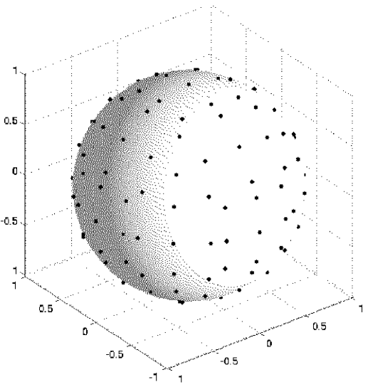
Figure 1: Unit sphere showing some of the $N_{d}=73$ directions over which the average is taken.

We have developed a less expensive technique for angle-averaging which does not require any 3-D interpolations. We first choose the vectors ${\bf r}_{j}$ from among those natural to a square computational grid. We restrict ourselves to the set of all unique directions which can be expressed with integer components with length less than or equal to $\sqrt{11}$. Let $j=1\cdots N_{d}$ be the index for this set. Each ${\bf r}_{j}$ is the minimum grid-point separation distance in the $j$th direction. This set is generated by the vectors (1,0,0), (1,1,0), (1,1,1), (2,1,0), (2,1,1), (2,2,1), (3,1,0) and (3,1,1) by taking all index and sign permutations of the three coordinates, and removing any vector which is a positive or negative multiple of any other vector in the set. This procedure generates a total of $N_{d}=73$ unique directions. The unit vectors associated with each direction are plotted as points on the sphere in Fig. 1. One can see that these points are well distributed over the sphere. Both the unit vectors $\hat{\bf r}_{j}$ and $-\hat{\bf r}_{j}$ are plotted, but below we do not consider the $-\hat{\bf r}_{j}$ directions since they give the same contribution as $\hat{\bf r}_{j}$ when averaged over the periodic computational domain.

For each of the $N_{d}$ directions, we form a set of $\ell=1\cdots N_{r}$ separation vectors, ${\bf x}_{i}+\ell{\bf r}_{j}$. Since ${\bf r}_{j}$ is the minimum separation distance of grid-points in the $j$th direction and $\ell$ is an integer, all the ${\bf x}_{i}+\ell{\bf r}_{j}$ lie on our computational grid. This is illustrated (in two-dimensions) for four directions in Fig. 2, where the black dots represent the points ${\bf x}_{i}+\ell{\bf r}_{j}$ and ${\bf x}_{i}$ is shown at the origin. We can now efficiently compute structure functions in $N_{d}$ different directions, at $N_{r}$ separation distances for each direction, without any 3-d interpolations:

$$\langle(\delta u_{L}(\ell{\bf r}_{j}))^{3}\rangle=\frac{1}{N^{3}}\sum_{i=1}^{N^{3}}\Big{[}\delta u_{L}(\ell{\bf r}_{j};{\bf x}_{i})\Big{]}^{3}.$$ (13)

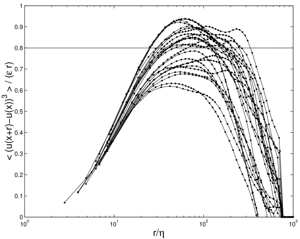
Figure 3: The third-order structure function normalized by $\varepsilon r$, computed from a single snapshot from the deterministic dataset. The dots indicate the values of the structure function computed at various $\ell{\bf r}_{j}$. Each thin curve is the cubic-spline interpolation through all computed values of the structure function in a particular direction. Only a few of the 73 different directions are shown here for visual clarity. The horizontal line indicates the 4/5ths mark.

For each direction, we get a 1-dimensional curve as a function of $\ell{\bf r}_{j}$, as shown in Fig. 3.

In the figure, points represent structure function values at the separation distances $\ell|{\bf r}_{j}|$, and each line is a cubic-spline fit to the data at $\ell=1\cdots N_{r}$ along each of the $N_{d}$ directions. One can see that only a few directions are computed at each of the separation distances, so we cannot directly take an angle-average from this data. But one can also see that the curves are quite smooth and the cubic-spline is an excellent interpolant. Thus we use cubic-spline interpolation to calculate the structure function in each of the $N_{d}$ directions, at separation vector $r\hat{\bf r}_{j}$ of any desired length $r$.

Once the data for each direction has been interpolated to a common separation distance $r$, we can approximate the angle-average at $r$ by quadrature over the $N_{d}$ directions:

$$\langle(\delta u_{L}(r))^{3}\rangle=\frac{1}{N_{d}}\sum_{j=1}^{N_{d}}w_{j}\langle(\delta u_{L}(r\hat{\bf r}_{j}))^{3}\rangle$$ (14)

In order to determine the quadrature weights $w_{j}$, we use the software package Stripack STRIPACK to compute the Voronoi tiling generated by the points ${\hat{\bf r}}_{j}$ on the unit sphere centered at ${\bf x}$. The weight $w_{j}$ is the solid angle subtended by the Voronoi cell containing the point ${\hat{\bf r}}_{j}$.

The angle-averaging procedure described can be implemented efficiently on parallel computers, requiring only the same type of parallel data transpose operator already used by a parallel pseudo-spectral code. The total cost of this angle-averaging procedure for one snapshot (73 directions and 100 different separation distances) is about the same as 150 timesteps of the Navier-Stokes code. Thus for a single eddy turnover time, where thousands of timesteps are required, the angle-averaging statistics can be computed during the computation with minimal impact on the total CPU time requirement.

III.1 Extracting the isotropic component

We first present results demonstrating how well the angle-average procedure performs at extracting the isotropic component from our DNS data. We again follow GFN02 and examine the relations between the second and third order velocity structure functions:

$$\langle(\delta u_{T})^{2}\rangle=(1+\frac{r}{2}\frac{d}{dr})\langle(\delta u_{L})^{2}\rangle$$ (15)

$$\langle\delta u_{L}(\delta u_{T})^{2}\rangle=\frac{1}{6}\frac{d}{dr}r\langle(\delta u_{L})^{3}\rangle$$ (16)

These equations require only isotropy and incompressibility. Thus in DNS data, where incompressibility is obtained to numerical round off error, deviations in the above relations are a measure of the anisotropy in the data. In GFN02 , the left and right sides of these equations are plotted after averaging in time. Excellent agreement is obtained in the inertial range, with some departure at larger scales.

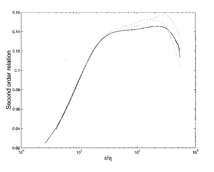
Figure 4: Second order isotropy relation for the stochastic dataset. Solid lines: left and right side of equation 15, normalized by $r^{2/3}$ and angle-averaged. Dotted lines: same quantities, only for a single coordinate direction.

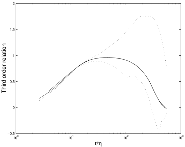
Figure 5: Third order isotropy relation for the deterministic dataset. Solid lines: left and right side of equation 16, normalized by $r$ and angle-averaged. Dotted lines: same quantities only for a single coordinate direction.

In Fig. 4, we show the second order isotropy relation for our stochastic dataset, and in Fig. 5 we show the third order relation for the deterministic dataset. This data is computed by angle-averaging over a single snapshot of the flow. The agreement is excellent, both in the inertial range and at the largest scales. For comparison, the figures also show the same relations from the same snapshot but using only a single coordinate direction instead of angle-averaging. In that case, there are significant differences for scales well into the inertial range. Thus the angle-averaging technique appears to be extremely effective in extracting the isotropic component of anisotropic data, even at large scales where anisotropy remains after time averaging over many snapshots. Similar results were obtained for the second order isotropy relation from the deterministic dataset and for the third order isotropy relation from the stochastic dataset.

III.2 Angle-averaging a single snapshot

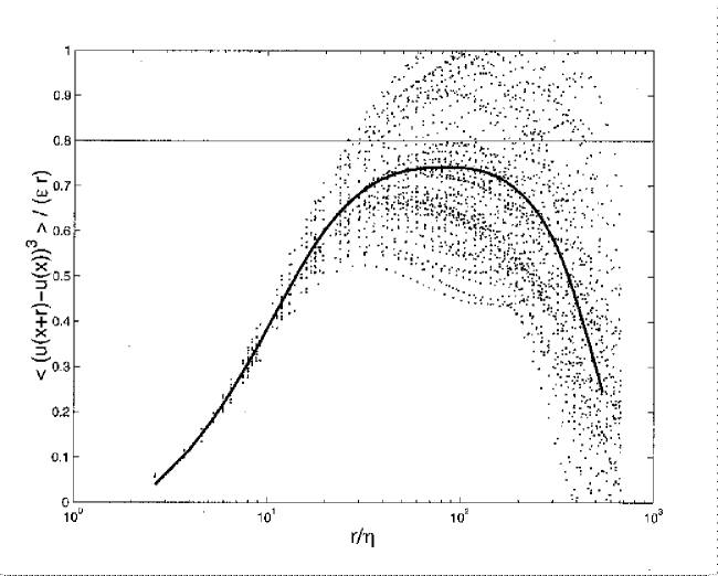
Figure 6: The third-order longitudinal structure function normalized by $\varepsilon r$, computed from a single snapshot of the stochastic dataset. The dots indicate the values of the structure function computed at various $\ell{\bf r}_{j}$. The thick curve is the angle-average. The horizontal line indicates the 4/5ths mark.

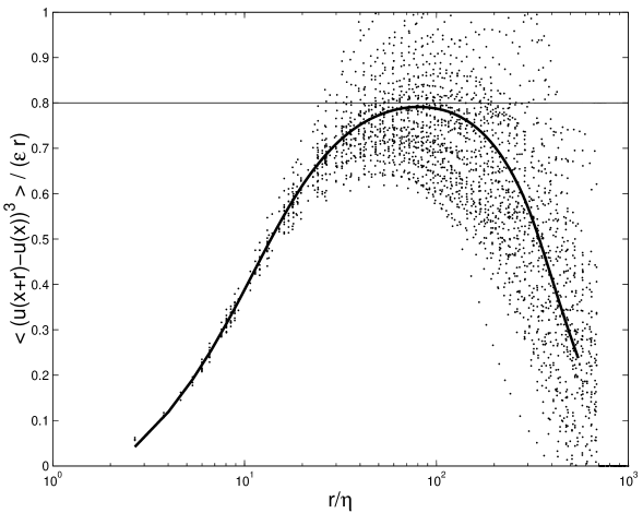
Figure 7: The third-order longitudinal structure function normalized by $\varepsilon r$, computed from a single snapshot of the deterministic dataset. The various symbols and lines mean the same as in Fig. 6.

We now present results from using angle-averaging to compute the third-order longitudinal structure function in the 4/5ths law. Figures 6 and 7 show the result of the angle-averaging procedure described above for single snapshots of the stochastic and deterministic datasets respectively. The snapshots are taken after the flow has had time to equilibrate. The value of the mean energy dissipation rate $\varepsilon$ was calculated from the snapshot. This is to be contrasted with previous works in which $\varepsilon$ is a long-time or ensemble average. We have therefore computed a version of the 4/5ths relation which is local in time. The dots represent the data from all 73 directions at all values of $r$ that were computed. The final weighted angle-average of Eq. (14) is given by the thick curves in both Figs. 6 and 7. One can see that the results from different directions are quite different, while the angle-averaged results are quite reasonable and similar to each other as well as similar to the results obtained from long time averaging of the coordinate directions presented in GFN02 and shown for our data in section III.4. Thus we conclude that angle-averaging the data from a single snapshot yields a very reasonable result. Similar results (not plotted) are obtained for the 4/3’rds and 4/15’ths laws.

III.3 Temporal variance

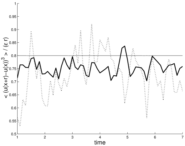
Figure 8: The angle-averaged (solid line) and single-direction (dotted line) values of the peak of the non-dimensionalized third-order longitudinal structure function for deterministic dataset, as a function of time.

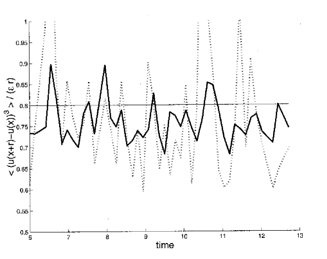
Figure 9: The angle-averaged (solid line) and single-direction (dotted line) values of the peak of the non-dimensionalized third-order longitudinal structure function for stochastic dataset, as a function of time.

To illustrate the variance in time of the third-order longitudinal structure function, with and without angle-averaging, we plot the peak value as a function of time for each dataset in Figures 8 and 9. The solid line is the angle-averaged value, and the dashed line is the value from a single coordinate direction. The angle-averaged value has a significantly reduced variance as compared to the single direction value, but one can see that there still is some variance from snapshot to snapshot. Thus in order to obtained fully converged statistics, some additional averaging is needed. In the next section we present results combining angle and time averaging.

Based on the local version of the K$41^{3}$ laws proved in DucRob99 ; Eyink02 , we expect that increasing the spatial resolution would allow us to obtain converged statistics from a single snapshot when used with angle-averaging. However, we could not expect such convergence without angle-averaging. This is because even in an isotropic flow, individual snapshots are not necessary isotropic - only the ensemble of all snapshots is guaranteed to be isotropic.

We note that the stochastic dataset (Fig. 9) shows a larger variation from snapshot to snapshot when compared to the deterministic dataset (Fig. 8). This is true for both the angle-averaged and single direction quantities shown in the figures, suggesting that the stochastic dataset produces data with a slightly larger variance in time, as expected.

III.4 Time averaged results

We now look at the 4/5ths law using both angle-averaging (which extracts the isotropic component of the statistics) and time-averaging (to remove the variance observed from snapshot to snapshot). The time-average is taken from 60 snapshots taken over 6 eddy turnover times. The results are shown in Fig. 10. The two datasets produce nearly identical results at all scales, even though the large scale forcing is quite different. The peak value of the stochastic and deterministic datasets are .755 and .752, respectively.

Thus we conclude that flows with similar geometry and Reynolds number have the same underlying isotropic component at all scales, at least up to third order statistics.

IV Conclusions

We have proposed a new, computationally efficient and easily implemented means of extracting isotropic statistics from an arbitrarily forced flow. As a first test of the method, we averaged the third-order structure functions over sufficiently many angles and discovered that the K$41^{3}$ relations are obtained, with tolerable variance, from a $single$ snapshot of homogeneous flow with either stochastic or deterministic forcing. This is a stronger result than was predicted by the original Kolmogorov ensemble approach or even the Nie-Tanveer version of NieTan99 . It appears that the results are, in fact, approaching the $local$ versions of K$41^{3}$ proposed in DucRob99 ; Eyink02 .

Using our procedure to extract the isotropic component, we are able to separate the effect of anisotropy from the effect of finite-Reynolds number on the statistics of the flow. This is an important point to make in the debate on how the two effects contaminate the inertial range. Once the anisotropy is eliminated, a more fruitful study of finite-Reynolds number effects can be made. It is clear from Fig. 10 that the Reynolds numbers are still not sufficient to give the wide inertial ranges that have been seen in high-Reynolds number experiments. However, it is also clear that angle-averaging has given a significant improvement in the results. With angle-averaging, less data is needed to obtain converged statistics, and deterministic forcings can be used without regard to the increased anisotropy they introduce.

The procedure we have described above can be used to investigate the isotropic component of higher-order structure functions or any other statistic as well. For example, the angle-averaged $n$th-order longitudinal structure functions may be measured in this way in order to determine scaling exponents which are truly independent of anisotropy. This method may also be used to isolate the anisotropic contributions themselves, as has been done in ABMP99 ; BLMT02 , by subtracting from the full structure function its angle-averaged value. Individual moments in a spherical harmonics expansion of structure functions can be computed by introducing the basis function of interest to the integrand in equation 14. In this way, the dominant scaling in anisotropic sectors can be determined, which is important to determine the rate of return to isotropy at small-scales. We plan to investigate such questions in future work.

Figure 2: Two dimensional example of how data is collected for the angle-averaging procedure. Four directions are shown, (1,0), (2,1), (3,1) and (1,1). Velocity data is known at all the grid points. The black dots represent values of $r$ where structure functions for a particular direction can be computed with no interpolations. Each structure function can then be interpolated to specific values of $r$, shown by the white dots.

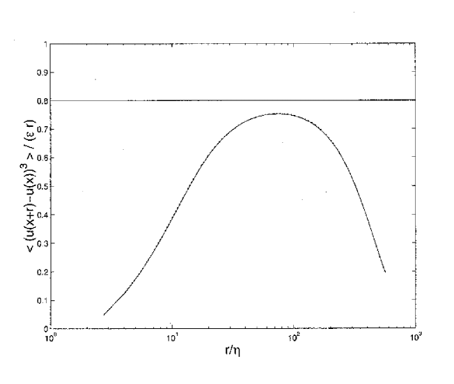
Figure 10: Time and angle-averaged third-order structure function normalized by $\varepsilon r$, for the deterministic dataset (solid line) and the stochastic dataset (dotted lines). The two curves are almost indistinguishable.

- (1) A.N. Kolmogorov, Doklad. Akad. Nauk. SSSR, 32 pp. 16–18 (1941). (Reproduced in Proc. Roy. Soc. Lond. A., 434 pp. 15–17, (1991)).
- (2) Monin and Yaglom, Statistical Fluid Mechanics II, Cambridge University Press, 1975.
- (3) K.R. Sreenivasan, S.I. Vainshtein, R. Bhiladvala, I. SanGil, S. Chen and N. Cao, Phys. Rev. Lett., 77 pp. 1488–1491 (1996).
- (4) M. R. Overholt and S. B. Pope, Comp. Fluids, 27 pp. 11–28 (1998).
- (5) N. P. Sullivan, S. Mahalingam, R. M. Kerr, Phys. Fluids, 6 pp. 1612–1614 (1994).
- (6) B. Dhruva, PhD Thesis, Yale University, 2001.
- (7) T. Gotoh, D. Fukayama and T Nakano, Phys. Fluids, 14 pp. 1065–1081 (2002).
- (8) Q. Nie and S. Tanveer, Proc. Roy. Soc. Lond. A, 455 pp. 1615–1635 (1999).
- (9) J. Duchon and R. Robert, Nonlinearity, 13 pp. 249–255, (2000).
- (10) G.L. Eyink, Nonlinearity, 16 pp. 137-145 (2003).
- (11) U. Frisch, Turbulence: The legacy of A.N. Kolmogorov, Cambridge University, (1995).
- (12) S. Kurien, K.R. Sreenivasan, Phys. Rev. E, 62 pp. 2206–2212 (2000).
- (13) I. Arad, B. Dhruva, S. Kurien, V.S. L’vov, I. Procaccia, K.R Sreenivasan, Phys. Rev. Lett., 81, pp. 5330–5333 (1998).
- (14) S. Kurien, V.S. L’vov, I. Procaccia, K.R Sreenivasan, Phys. Rev. E, 61 pp. 407–421 (2000).
- (15) I. Arad, V.S. L’vov, I. Procaccia, Phys. Rev. E, 59 pp. 6753–6765 (1999).
- (16) S. Kurien and K.R. Sreenivasan, “Measures of Anisotropy and the Universal Properties of Turbulence”, New Trends in Turbulence, Les Houches Summer School 2000, Eds: M. Lesieur, A. Yaglom, F. David, pp. 53–109 (2002).
- (17) I. Arad, L. Biferale, I. Mazzitelli, I. Procaccia, Phys. Rev. Lett, 82 pp. 5040–5043 (1999).
- (18) L. Biferale, D. Lohse, I.M. Mazzitelli, P. Toschi, J. Fluid Mech, 452 pp. 39–59 (2002).
- (19) R. Renka, Algorithm 772: STRIPACK, Delaunay Triangulation and Voronoi Diagram on the Surface of a Sphere, ACM Trans. Math. Software 23 (1997). http://www.math.iastate.edu/burkardt/f_src/stripack/stripack.html