Instabilities in the two-dimensional cubic nonlinear Schrödinger equation

Abstract

The two-dimensional cubic nonlinear Schrödinger equation (NLS) can be used as a model of phenomena in physical systems ranging from waves on deep water to pulses in optical fibers. In this paper, we establish that every one-dimensional traveling wave solution of NLS with trivial phase is unstable with respect to some infinitesimal perturbation with two-dimensional structure. If the coefficients of the linear dispersion terms have the same sign then the only unstable perturbations have transverse wavelength longer than a well-defined cut-off. If the coefficients of the linear dispersion terms have opposite signs, then there is no such cut-off and as the wavelength decreases, the maximum growth rate approaches a well-defined limit.

I Introduction

The two-dimensional cubic nonlinear Schrödinger equation (NLS) is given by

$$i\psi_{t}+\alpha\psi_{xx}+\beta\psi_{yy}+\gamma|\psi|^{2}\psi=0,$$ (1)

where $\psi=\psi(x,y,t)$ is a complex-valued function, and $\alpha$, $\beta$ and $\gamma$ are real constants. Among many other situations, NLS arises as an approximate model of the evolution of a nearly monochromatic wave of small amplitude in pulse propagation along optical fibers Manakov (1974) where $\alpha\beta>0$, in gravity waves on deep water Benney and Roskes (1969) Davey and Stewartson (1974) where $\alpha\beta<0$ and in Langmuir waves in a plasma Pecseli (1985) where $\alpha\beta>0$. As a description of a superfluid Donnelly (1991), NLS is known as the Gross-Pitaevskii equation Gross (1963) Pitaevskii (1961) with $\alpha\beta>0$. Sulem and Sulem Sulem and Sulem (1999) examine NLS in detail.

NLS admits a large class of one-dimensional traveling wave solutions of the form

$$\psi(x,y,t)=\phi(ax+by-st)\mbox{e}^{i\lambda t+ia\bar{s}x+ib\bar{s}y+i\eta},$$ (2)

where $\phi$ is a real-valued function, $\bar{s}=s/(2\alpha a^{2}+2\beta b^{2})$ and $a$, $b$, $s$, $\lambda$ and $\eta$ are real parameters. By making use of the symmetries of NLS Sulem and Sulem (1999), all solutions of this form can be considered by studying the simplified form

$$\psi(x,y,t)=\phi(z)\mbox{e}^{i\kappa x+i\lambda t},$$ (3)

where $\phi$ is a real-valued function, $z=x-2\alpha\kappa t$, and $\kappa$ and $\lambda$ are real parameters.

If $\alpha\gamma>0$, then NLS admits the following two solutions of the form (3)

$$\phi(z)=\sqrt{2\frac{\alpha}{\gamma}}\;k\;\mbox{cn}(z,k),\;\;\text{with}\;\;\lambda=\alpha(2k^{2}-1-\kappa^{2}),$$ (4)

$$\phi(z)=\sqrt{2\frac{\alpha}{\gamma}}\;\mbox{dn}(z,k),\;\;\text{with}\;\;\lambda=\alpha(2-k^{2}-\kappa^{2}).$$ (5)

If $\alpha\gamma<0$, then NLS admits the following solution

$$\phi(z)=\sqrt{-2\frac{\alpha}{\gamma}}\;k\;\mbox{sn}(z,k),\;\text{with}\;\lambda=-\alpha(1+k^{2}+\kappa^{2}).$$ (6)

Here $k\in[0,1]$ is a free parameter known as the elliptic modulus and $\mbox{cn}(\cdot,k)$, $\mbox{dn}(\cdot,k)$, and $\mbox{sn}(\cdot,k)$ are Jacobi elliptic functions. Byrd and Friedman Byrd and Friedman (1954) provide a complete review of elliptic functions. If $k<1$, then each function $\phi(z)$ is periodic. As $k\rightarrow 1$, the period of each increases without bound, and $\phi(z)$ limits to an appropriate hyperbolic function, which we call a “solitary wave.”

These solutions, plus the “Stokes’ wave” (plane wave)

$$\psi(x,t)=A\mbox{e}^{i\kappa x-i(\alpha\kappa^{2}-\gamma|A|^{2})t},$$ (7)

comprise the entire class of bounded traveling wave solutions of NLS with trivial phase Carr et al. (2000). Davey and Stewartson Davey and Stewartson (1974) show that a Stokes’ wave is unstable unless either $\alpha\beta\gamma=0$, or $\alpha\beta>0$ and $\alpha\gamma<0$. In the remainder of this paper, we concentrate on (4), (5) and (6), and on their instabilities.

Zakharov and Rubenchik Zakharov and Rubenchik (1974) establish that (4) and (5) with $k=1$ are unstable with respect to long-wave transverse perturbations. Pelinovsky Pelinovsky (2001) reviews the stability of solitary wave solutions of NLS with $\alpha\beta<0$ and $\alpha\gamma>0$, and presents an analytical expression for the growth rate of the instability near a cut-off. Extensive reviews of the stability of solitary wave solutions are given in Kuznetsov et al. (1986); Rypdal and Rasmussen (1989); Kivshar and Pelinovsky (2000). The periodic problem has not been studied in as much detail, though Martin, Yuen and Saffman Martin et al. (1980) examine numerically the stability of the solution given in (5) for a range of parameters.

We present four main results in this paper. First, every one-dimensional traveling wave with trivial phase is unstable with respect to some infinitesimal perturbation with two-dimensional structure. For all choices of the parameters, there are unstable perturbations with long transverse wavelength. This generalizes the result of  Zakharov and Rubenchik (1974).

Second, if $\alpha\beta>0$, then the only unstable perturbations have transverse wavelength longer than a well-defined cut-off.

Third, if $\alpha\beta<0$, then there is no such cut-off. There are unstable perturbations with arbitrarily short wavelengths in both transverse and longitudinal directions. These short wavelength instabilities seem to have been overlooked in previous analyses.

Fourth, for $\alpha\beta<0$, the unstable perturbations with short wavelength have transverse wavenumbers that are confined to narrower and narrower intervals as the transverse wavenumber grows without bound. In these unstable intervals, as the transverse wavenumber grows without bound, the maximum growth rate approaches a well-defined limit. As $k\rightarrow 1$, this limiting growth rate tends to zero if $\alpha\gamma>0$, and to a finite non-zero limit if $\alpha\gamma<0$.

II Stability Analysis

We consider perturbed solutions, $\psi_{{}_{p}}=\psi_{{}_{p}}(x,y,t)$, with the following structure

$$\psi_{{}_{p}}=(\phi(z)+\epsilon u(x,y,t)+i\epsilon v(x,y,t)+O(\epsilon^{2}))\mbox{e}^{i\kappa x+i\lambda t},$$ (8)

where $u(x,y,t)$ and $v(x,y,t)$ are real-valued functions, $\epsilon$ is a small real parameter, $z=x-2\alpha\kappa t$, and $\phi(z)\mbox{e}^{i\kappa x+i\lambda t}$ is one of the solutions presented in the previous section. Substituting (8) into (1), linearizing and separating into real and imaginary parts gives

$$-(\alpha\kappa^{2}+\lambda)u+3\gamma\phi^{2}u+\beta u_{yy}+\alpha u_{xx}=v_{t},$$ (9a)

$$-(\alpha\kappa^{2}+\lambda)v+\gamma\phi^{2}v+\beta v_{yy}+\alpha v_{xx}=-u_{t}.$$ (9b)

Without loss of generality, assume that $u(x,y,t)$ and $v(x,y,t)$ have the forms

$$u(x,y,t)=U(z,\rho)\mbox{e}^{i\rho y-\Omega t}+c.c.,$$ (10a)

$$v(x,y,t)=V(z,\rho)\mbox{e}^{i\rho y-\Omega t}+c.c.,$$ (10b)

where $\rho$ is a real constant, $\Omega$ is a complex constant, $U$ and $V$ are complex-valued functions and $c.c.$ denotes complex conjugate. This leads to

$$(\alpha\kappa^{2}+\lambda)U-3\gamma\phi^{2}U+\beta\rho^{2}U-\alpha\partial_{z}^{2}U=\Omega V,$$ (11a)

$$(\alpha\kappa^{2}+\lambda)V-\gamma\phi^{2}V+\beta\rho^{2}V-\alpha\partial_{z}^{2}V=-\Omega U.$$ (11b)

These are the central equations in this paper. We assume that $U$ and $V$ are periodic with the same period as $\phi$. More general boundary conditions are discussed in Carter (2001). Instability occurs if (11b) admits a periodic solution with $Re(\Omega)<0$. Without loss of generality, for the remainder of this paper we assume $\kappa=0$ by redefining $\lambda$.

In Sections III and IV, we examine (11b) using small-$\rho$ and large-$\rho$ asymptotic analyses respectively. In Section V, we present results from a numerical study in which (11b) was solved for a wide range of $\rho$ values.

III Small-$\rho$ limit

Generalizing the work in Zakharov and Rubenchik (1974), we assume that for fixed $k$ and for fixed small $\rho$, (11b) admits solutions of the form

$$U\sim u_{0}(z)+\rho u_{1}(z)+\rho^{2}u_{2}(z)+\cdots,$$ (12a)

$$V\sim v_{0}(z)+\rho v_{1}(z)+\rho^{2}v_{2}(z)+\cdots,$$ (12b)

$$\Omega^{2}\sim\rho^{2}\omega_{1}+\rho^{3}\omega_{2}+\cdots,$$ (12c)

where the $\omega_{j}$ are complex constants and the $u_{j}$ and $v_{j}$ are complex-valued periodic functions with the same period as $\phi$.

This assumption leads to the “neck” mode

$$U_{n}(z,\rho)=O(\rho),$$ (13a)

$$V_{n}(z,\rho)=\phi+O(\rho),$$ (13b)

$$\Omega_{n}^{2}=-\alpha\beta\rho^{2}\omega_{1n}+O(\rho^{3}),$$ (13c)

and the “snake” mode

$$U_{s}(z,\rho)=\frac{d\phi}{dz}+O(\rho),$$ (14a)

$$V_{s}(z,\rho)=O(\rho),$$ (14b)

$$\Omega_{s}^{2}=-\alpha\beta\rho^{2}\omega_{1s}+O(\rho^{3}),$$ (14c)

where $\omega_{1n}$ and $\omega_{1s}$ are functions of the elliptic modulus of the unperturbed solution. Complicated but exact expressions for $\omega_{1n}$ and $\omega_{1s}$ are derived in Carter (2001). The final results are presented in Fig. 1, where we plot $\omega_{1n}$ and $\omega_{1s}$, the growth rates, versus $k$ for (4), (5) and (6).

These plots establish that $\omega_{1n}<0$ for (4) and (5) and $\omega_{1s}<0$ for (6). Therefore, if $\alpha\beta>0$, (4) and (5) are unstable with respect to long-wave transverse perturbations corresponding to the neck mode and (6) is unstable with respect to long-wave transverse perturbations corresponding to the the snake mode.

These plots also establish that $\omega_{1s}>0$ for (4) and (5) and $\omega_{1n}>0$ for (6). Therefore, if $\alpha\beta<0$, (4) and (5) are unstable with respect to the snake mode and (6) is unstable with respect to the neck mode.

It follows from these results that a trivial-phase solution of NLS is unstable to a growing neck mode if $\beta\gamma>0$, and to a growing snake mode if $\beta\gamma<0$.

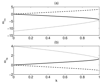
Figure 1: Plots of $\omega_{1n}$ and $\omega_{1s}$ versus $k$ in (a) and (b) respectively. The solid line corresponds to (4), the dotted line corresponds to (5) and the dashed line corresponds to (6).

IV Large-$\rho$ limit

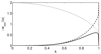
Figure 2: Plots of $-w_{min}/|\alpha|$ versus $k$. The solid line corresponds to (4), the dotted line corresponds to (5) and the dashed line corresponds to (6).

If $\alpha\beta>0$ and $\rho$ is chosen to be large enough to satisfy

$$\rho^{2}>5|\frac{\alpha}{\beta}|,$$ (15)

then the two operators on the left side of (11b) have the same sign, so $\Omega^{2}<0$. Therefore, there is no large-$\rho$ instability if $\alpha\beta>0$.

If $\alpha\beta<0$ and $\rho$ is large, then one can show that there is no instability unless $\Omega=O(1)$. Therefore, we assume

$$U\sim\zeta_{1}(\mu z)+\rho^{-2}\zeta_{2}(\mu z)+\cdots,$$ (16a)

$$V\sim\xi_{1}(\mu z)+\rho^{-2}\xi_{2}(\mu z)+\cdots,$$ (16b)

$$\Omega\sim w_{1}+\rho^{-2}w_{2}+\cdots,$$ (16c)

$$\alpha\mu^{2}=-\beta\rho^{2}+\nu+O(\rho^{-2}),$$ (16d)

where $\nu$ is a real constant, the $w_{j}$ are complex constants, and the $\zeta_{j}$ and $\xi_{j}$ are complex-valued periodic functions with the same period as $\phi$.

Substituting (16d) into (11b), one finds at leading order

$$U\sim\zeta_{11}\sin(\mu z+z_{0})+O(\rho^{-2}),$$ (17a)

$$V\sim\xi_{11}\sin(\mu z+z_{0})+O(\rho^{-2}),$$ (17b)

where $\zeta_{11}$, $\xi_{11}$ and $z_{0}$ are constants. Requiring $U$ and $V$ to have the same period as $\phi(z)$ forces $\mu$ to take on discrete values: $\mu=2\pi N/L$, where $L$ is the period of $\phi(z)$, and $N$ is an integer. To satisfy (16d), $N\gg 1$. At the next order in $\rho$, solutions are periodic only if

$$w_{1}=\pm\sqrt{\gamma f-\lambda+\nu}\sqrt{\lambda-3\gamma f-\nu},$$ (18)

where $f$ is the Fourier coefficient (in $\sin(\mu z+z_{0})$) of $\phi^{2}(z)\sin(\mu z+z_{0})$ and $\nu$ is $O(1)$ but otherwise arbitrary. Minimizing the negative root in (18) with respect to $\nu$ leads to

$$w_{min}=-|\gamma f|,$$ (19)

when $\nu=(\lambda-2\gamma f)$. Then (16d) defines $\rho_{{}_{N}}$, the value of $\rho$ at which the Nth unstable mode achieves its maximum growth rate:

$$-\beta\rho^{2}_{{}_{N}}=\alpha(2\pi N/L)^{2}+2\gamma f-\lambda.$$ (20)

We also find how for $\rho$ can deviate from $\rho_{{}_{N}}$ before $\Omega^{2}$ becomes negative

$$\delta\rho_{{}_{N}}\sim|\gamma|f/(2|\beta|\rho_{{}_{N}})=O(1/N),\quad\text{for}\quad N\gg 1.$$ (21)

Analytic expressions for the $f$ corresponding to the solutions given in (4), (5) and (6) are not known. But, in the large-$\rho$ limit, the Riemann-Lebesgue Lemma Guenther and Lee (1988) can be used to determine approximate expressions. As $\rho\rightarrow\infty$, for the solution given in (4),

$$f\sim\frac{1}{2K(k)}\big{|}\frac{\alpha}{\gamma}\big{|}\Big{(}E(\mbox{am}(4K(k)))+4(k^{2}-1)K(k)\Big{)},$$ (22)

for the solution given in (5),

$$f\sim\frac{1}{K(k)}\big{|}\frac{\alpha}{\gamma}\big{|}\Big{(}E(\mbox{am}(2K(k)))\Big{)},$$ (23)

and for the solution given in (6),

$$f\sim\frac{1}{2K(k)}\big{|}\frac{\alpha}{\gamma}\big{|}\Big{(}4K(k)-E(\mbox{am}(4K(k)))\Big{)}.$$ (24)

In each of these expressions, $\mbox{am}(\cdot)$ gives the Jacobi amplitude and $K(\cdot)$ and $E(\cdot)$ are the complete elliptic integrals of the first and second kind respectively Byrd and Friedman (1954).

Plots of $-w_{min}/|\alpha|$, a growth rate, versus $k$ are given in Fig. 2. This argument establishes that all finite-period one-dimensional trivial phase solutions are unstable with respect to arbitrarily short-wavelength transverse perturbations if $\alpha\beta<0$, and that the growth rate of the instability remains bounded as $\rho\rightarrow\infty$.

Note that as $k\rightarrow 1$, $\phi(z)$ in (6) approaches a hyperbolic tangent and the growth rate approaches that of the Stokes’ wave with an amplitude of $\sqrt{-2\alpha/\gamma}$. This establishes that there are an infinite number of of unstable branches if $\alpha\beta<0$ and $\alpha\gamma<0$.

Also note that as $k\rightarrow 1$, $\phi(z)$ in both (4) and (5) approaches a hyperbolic secant, and the corresponding growth rate limits to zero. This establishes that there is no large-$\rho$ instability in the solitary wave limit if $\alpha\gamma>0$.

V Monodromy

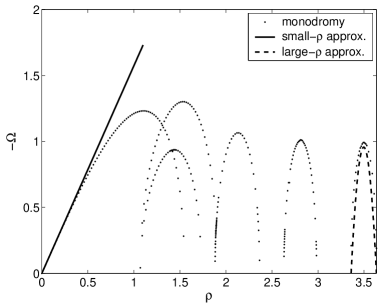
Figure 3: Plots of $-\Omega$ versus $\rho$ corresponding to (4) with
$k=\sqrt{0.8}$ and $-\alpha=\beta=\gamma=1$. See text for a description.

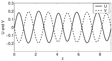
Figure 4: Plots of $U$ and $V$ versus $z$ corresponding to $(\rho=3.5,\Omega=-0.99,N=5)$.

The system of equations in (11b) is Hamiltonian in $z$, with periodic boundary conditions. The coordinates on the phase space are $p_{1}=dU/dz$, $p_{2}=-dV/dz$, $q_{1}=U$ and $q_{2}=V$. The Hamiltonian is

$$H=\frac{1}{2}(p_{1}^{2}-p_{2}^{2})-\frac{1}{2\alpha}(\lambda+\beta\rho^{2}-3\gamma\phi^{2}(x))q_{1}^{2}$$

$$+\frac{1}{2\alpha}(\lambda+\beta\rho^{2}-\gamma\phi^{2})q_{2}^{2}+\frac{\Omega}{\alpha}q_{1}q_{2}.$$ (25)

Such a Hamiltonian system necessarily has a monodromy structure with invariants Meyer and Hall (1992). We used this structure to identify the periodic solutions of (11b) by numerically integrating (11b) over one period of $\phi$.

The growth rates obtained from numerical simulations corresponding to (6) with $k=\sqrt{0.8}$ and $-\alpha=\beta=\gamma=1$ are included in Fig. 3 as dots. The line is obtained from the small-$\rho$ results. The dashed curve is obtained from the large-$\rho$ results with $N=5$. Each dotted curve corresponds to a different unstable mode. A plot of the spatial structure of the mode corresponding to $(\rho=3.5,\Omega=-0.99,N=5)$ is given in Fig. 4.

Figure 3 demonstrates strong agreement between the numerical results and the small-$\rho$ analysis when $\rho$ is near zero. It also demonstrates agreement between the numerical results and the large-$\rho$ analysis.

Figure 4 demonstrates that the $U$ and $V$ obtained numerically are similar in form to the $U$ and $V$ obtained in the large-$\rho$ analysis.

This work was supported by National Science Foundation Grants DMS-9731097, DMS-98-10751, and DMS-0139771. We acknowledge useful discussions with Bernard Deconinck and Nathan Kutz.

References

- Manakov (1974) S. V. Manakov, Sov Phys JETP 38, 248 (1974).
- Benney and Roskes (1969) D. J. Benney and G. J. Roskes, Stud in Appl Math 48, 377 (1969).
- Davey and Stewartson (1974) A. Davey and K. Stewartson, Proc R Soc London Ser A 338, 101 (1974).
- Pecseli (1985) H. L. Pecseli, IEEE Transactions Plasma Science 13, 53 (1985).
- Donnelly (1991) R. Donnelly, Quantized Vortices in Helium II (Cambridge University, England, 1991).
- Gross (1963) E. P. Gross, J Math Phys 4, 195 (1963).
- Pitaevskii (1961) L. P. Pitaevskii, Sov Phys JETP 13, 451 (1961).
- Sulem and Sulem (1999) P. L. Sulem and C. Sulem, Nonlinear Schrödinger Equations: Self-focusing and Wave Collapse (Springer, New York, 1999).
- Byrd and Friedman (1954) P. F. Byrd and M. D. Friedman, Handbook of Elliptic Integrals for Engineers and Physicists (Springer-Verlag, 1954).
- Carr et al. (2000) L. D. Carr, C. W. Clark, and W. P. Reinhardt, Phys Rev A 62, 63610 (2000); 62, 63611 (2000).