Filament bifurcations in a one-dimensional model of reacting excitable fluid flow

Abstract

Recently, it has been shown that properties of excitable media stirred by two-dimensional chaotic flows can be properly studied in a one-dimensional framework [8, 9], describing the transverse profile of the filament-like structures observed in the system. Here, we perform a bifurcation analysis of this one-dimensional approximation as a function of the Damköhler number, the ratio between the chemical and the strain rates. Different branches of stable solutions are calculated, and a Hopf bifurcation, leading to an oscillating filament, identified.

1 Introduction

Chemically reacting substances in fluid flows are complex systems important both from a fundamental point of view and for its relevance in industrial and environmental contexts [1, 2]. Typical incompressible chaotic flows stretch fluid parcels along particular directions, with the consequent contraction along the others. Thus, passive markers draw filamental or lamellar structures that have been investigated both from theory as from experiment[3, 4]. Chemical reactants are also stretched in this way, producing a great increase in the surface of contact between different species with deep effects on the global chemical kinetics[5]. In addition to the strictly chemical interactions, biological interactions in ecosystems (predation, grazing, consumption, competition, …) can also be described in the same framework, so that stability and dynamics of aquatic ecosystems are also strongly influenced by this filamentation process[6].

In this Paper we analyze a simplified model describing the transverse chemical structure of these filaments, for the case in which the chemical or biological activity is of the excitable type. This includes in particular well known laboratory reactions, such as the Belousov-Zhabotinsky reaction, but also reactions of environmental importance, such as phytoplankton-zooplankton competition[7]. Such kind of dynamics in two-dimensional chaotic flows was analyzed in [8, 9]. There it was found that some of the dynamic regimes and transitions between them can be understood in terms of a simple one-dimensional model, of the kind already considered in [10, 11, 12, 13] that focusses in the transverse structure of the filaments. It was mentioned in [9] that, in addition to the bifurcations considered there in detail, there was a range of parameters for which a complex coexistence of solutions and bifurcations occurred, that may be of relevance to understand qualitative behaviors of the two-dimensional chaotic flows. The present paper focusses in that regime. We use the FitzHug-Nagumo model as a prototypical excitable dynamics, but we expect that the same qualitative results will be also obtained for other chemical or biological excitable schemes. Similar behavior has been observed in an excitable model of oceanic plankton population in [14].

2 The one-dimensional filament model

Given a set of kinetic laws describing the time evolution of a number of chemical or biological concentrations $\{C_{i}({\bf x},t)\}_{i=1,...,N}$ in a homogeneous system,

$${dC_{i}\over dt}=kF_{i}(C_{1},...,C_{N})\ \$$ (1)

($k$ is a global reaction rate), a general partial differential equation model describing their spatiotemporal evolution under the simultaneous additional effects of advection in an incompressible velocity field ${\bf v}({\bf x},t)$, and diffusion with diffusion coefficients $\{D_{i}\}$, is the one given by the following advection-reaction-diffusion equations:

$${\partial C_{i}({\bf x},t)\over\partial t}+{\bf v}({\bf x},t)\cdot\nabla C_{i}({\bf x},t)=kF_{i}(C_{1},...,C_{N})+D_{i}\nabla^{2}C_{i}({\bf x},t)\ \ .$$ (2)

In the following we restrict for simplicity to the case of equal diffusion coefficients $D_{i}=D,\ \forall i$. In the immediate vicinity of filaments or lamelae, one can approximate the flow by its linearization around a point co-moving with a fluid element. In areas where the advection dynamics is hyperbolic this linearization identifies principal directions $\{x_{j}\}$ along which the corresponding velocity components read $v_{j}=\lambda_{j}x_{j}$. Positive and negative values of the strain rate $\lambda_{j}$ identify expanding and contracting directions, respectively. Along the expanding directions, diffusion and advection cooperate and the chemical concentrations are fastly homogenized, whereas strong gradients build-up in the contracting directions. This is the origin of filamental (one expanding direction) or lamellar (two expanding directions) structures. Gradients in Eq. (2) can be safely neglected except along the contracting directions. We consider here the case of filaments in two-dimensional flows, or lamellae in three dimensions, so that there is only one contracting direction, of strain rate $\lambda_{i}\equiv-\lambda$, with $\lambda>0$. In this case, (2) reduces to an effective one-dimensional model for the transverse profile of the chemical distributions. By measuring time in units of $\lambda^{-1}$, and space in units of $\sqrt{D/\lambda}$, we arrive at:

$${\partial C_{i}(x,t)\over\partial t}-x{\partial\over\partial x}C_{i}(x,t)={\rm Da}F_{i}(C_{1},...,C_{N})+{\partial^{2}\over\partial x^{2}}C_{i}(x,t)\ \ .$$ (3)

We have introduced a Damköhler number ${\rm Da}=k/\lambda$ as the ratio between the chemical and the strain rate.

Several limitations are inherent to (3). It is a strictly local model valid close to (moving) hyperbolic trajectories. The linearization assumption will only be justified if the full filament width is smaller than any structure in the velocity field. This implies in particular a very small diffusion coefficient so that we are deeply in the Batchelor regime. Additional qualitative changes of behavior, not contained in (3), are expected when increasing the diffusion coefficient in (2). Curvature effects or, more importantly, any interaction between filaments, are completely neglected. Finally, the use of a constant $\lambda$ neglects any fluctuations of the stretching rate.

The FitzHugh-Nagumo (FN) model consists in a dynamics of the type (1) for two interacting species, of concentrations $C_{1}$ and $C_{2}$, and reaction terms:

$$F_{1} = C_{1}(a-C_{1})(C_{1}-1)-C_{2},$$ (4)

$$F_{2} = \epsilon(C_{1}-\gamma C_{2}).$$ (5)

The FN model behaves excitably when $\epsilon\ll 1$ so that there is a separation between the fast evolution of the active component or activator, $C_{1}$, and the slow evolution of $C_{2}$, the passive one or inhibitor. We concentrate in the parameter values $\epsilon=10^{-3}$, $\gamma=3.0$, and $a=0.25$, for which robust excitable behavior is obtained.

3 Filament solutions

The unexcited solution, $C_{1}=C_{2}=0$, is a linearly stable exact solution of system (3)-(5). In addition, the most notable solution is a pulse like steady solution, centered on $x=0$, in which the activator is fully excited in a central region, whereas the inhibitor remains at reduced concentrations. This chemical distribution can be thought as the transverse cut of one of the excited filaments seen in two-dimensional excitable fluid flows. Pulse solutions of this type are shown in Fig. 1.

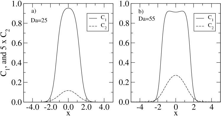
Figure 1: One-hump solutions for the two chemical components: $C_{1}$ and $C_{2}$ (multiplied by a factor $5$); a) ${\rm Da}=25$; b) ${\rm Da}=55$.

The width, $w_{s}$, of this solution is determined by the competition between the tendency to expand, due to the joint effects of the excitable chemistry and diffusion, and the compression by the flow, and can be estimated [8, 9] to be, for small $\epsilon$, $w_{s}\approx(1-2a)\sqrt{{\rm Da}/2}$. It is very similar to what is obtained in one-component bistable chemical models[12], so that the presence of the inhibitor plays here only a secondary rôle.

As in bistable chemical models, this stable pulse solution coexists in a range of parameters with a unstable pulse, of width given at small $\epsilon$ approximately by [9] $w_{u}\approx 2/\sqrt{a{\rm Da}}$. When the value of ${\rm Da}$ decreases (meaning that the chemistry becomes slower, or the stretching faster) the two solutions approach, collide and disappear from phase space in a saddle-node bifurcation [9]. This happens at a value of ${\rm Da}_{c}\approx 2\sqrt{2/a}(1-2a)^{-1}$. Thus, the excited pulse solution does not exists at small ${\rm Da}$, and the existence of a critical ${\rm Da}_{c}$ explains [9] the dynamical transition occurring in closed two-dimensional chaotic flows between a situation in which local perturbations of the unexcited state have limited impact on the system, and a state in which they give rise to a global excitation of the whole fluid. A related transition occurs in open flows [9].

At larger values of ${\rm Da}$, the influence of the inhibitor becomes more noticeable and, as a result, steady filament solutions have a ‘two-humped’ shape (Fig.2a). It was noted in [9] that this kind of ‘double-filament’, also seen in two-dimensional flow simulations, can be regarded as a bound state of two asymmetric counter-propagating excitable pulses, which are also steady solutions of model (3)-(5) coexisting with the symmetric ones at large ${\rm Da}$ (Fig. 2b). Of course, for each value of ${\rm Da}$ there are two asymmetric solutions of this kind, each one being the specular image of the other.

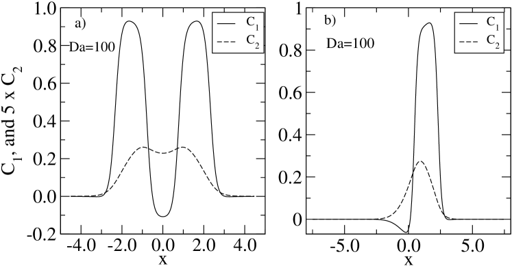
Figure 2: Two types of pulses for ${\rm Da}=100$: a) The two-hump symmetric solution; b) the asymmetric one.

4 Bifurcation behavior at intermediate Da

It was noted in [9] that a complex bifurcation scenario occurred between the small and the large values of ${\rm Da}$ for which the solutions in Figs. (1) and (2) were respectively obtained. It happens that these three solution branches are not directly connected, at least for the values of $\epsilon$ and $\gamma$ considered here. We have followed the three branches of steady stable pulse solutions by starting with well developed solutions at large and small ${\rm Da}$, and then performing slow changes in ${\rm Da}$. In this way we can only follow stable solutions. A more complete characterization would require also the continuation of unstable branches, that will be performed elsewhere. We monitor the height of the activator at $x=0$, and plot it in Fig. 3.

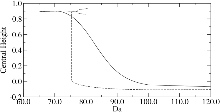
Figure 3: Bifurcation diagram for the system given by Eq. (3). We plot the height of stable solutions in terms of ${\rm Da}$. Solid line corresponds to decreasing the value of ${\rm Da}$ from an initial state of the asymmetric type, like that in Fig. 2b), at large ${\rm Da}$. Dashed line is obtained in the same way but beginning from a symmetric two-hump pulse (Fig.2a). Dashed-dotted line is obtained increasing the value of ${\rm Da}$ from a symmetric one-hump pulse (Fig.1a)).

When increasing the value of ${\rm Da}$ on the symmetric one-humped solution branch, the inhibitor value increases in the center, so that for ${\rm Da}\gtrsim 45$, the central concentration of the activator becomes a shallow minimum (Fig. 1b). So, above this parameter value, this branch can be called ‘slightly two-humped’, and it remains so until $Da\approx 77.1$. It is however clearly different from the ‘strongly two-humped’ solution branch to which Fig. 2a pertains. At $Da\approx 77.1$, a Hopf bifurcation occurs: the filament (both the $C_{1}$ and the $C_{2}$ concentrations) pulsates in height, width and shape. We show in Fig. (4) this behavior. For ${\rm Da}$ above this Hopf bifurcation, we plot in Fig. 3 the maximum and minimum central height values attained during the oscillation. At ${\rm Da}\approx 81.0$ the width becomes too narrow at some moment of the oscillation and the filament collapses to the unexcited ($C_{1}=C_{2}=0$) solution, so that the limit cycle solution disappears. This collapse probably reveals the collision of the filament limit cycle with an unstable pulse solution that we have not characterized. The basin of attraction of the oscillating solution is rather narrow: at these values of ${\rm Da}$ it is easier to be attracted by the two-hump symmetric steady solution branch or the unexcited state.

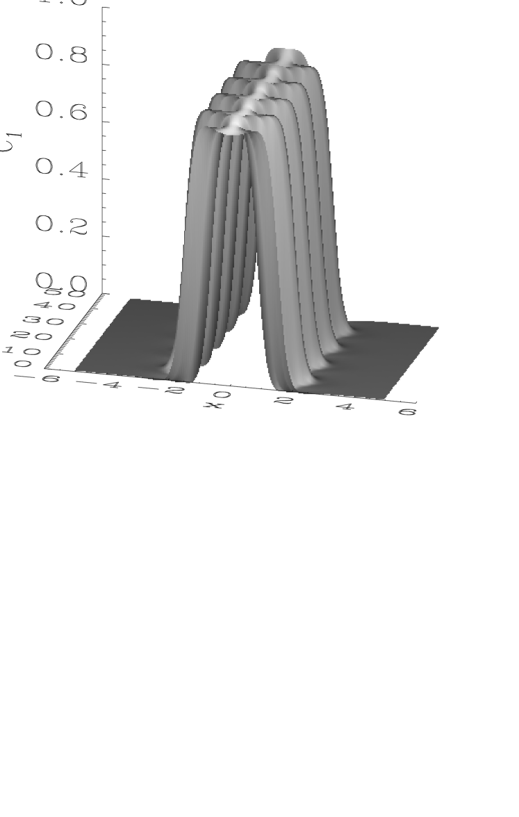
Figure 4: Spatio-temporal plot of $C_{1}$ in an oscillating filament at ${\rm Da}=79$.

On the other hand, if we start with a well developed two-hump filament such as the one in Fig. 2a at high ${\rm Da}$, the two humps approach each other when decreasing ${\rm Da}$. Before they fuse together, there is a discontinuous jump (at ${\rm Da}\approx 75.4$) to the steady ‘slightly two-humped filament’ followed before. This probably reveals a saddle-node bifurcation in which the stable two-hump branch collides with an unstable one, that we have not followed.

Finally, starting from the asymmetric filament of Fig. 2b, it approaches the $x=0$ axis when decreasing ${\rm Da}$, becoming more and more symmetric. For the values of $\epsilon$ and $\gamma$ used here, however, it does not join smoothly with the symmetric branch in a forward pitchfork bifurcation in which it would also join the other asymmetric filament of opposite symmetry. Rather, it performs a (small) discontinuous jump to the symmetric filament branch at ${\rm Da}\approx 70.48$. This is probably the signature of a backward pitchfork bifurcation, or of some other complex coexistence with unstable solutions, that would also explain the observed range of bistability between the symmetric and asymmetric filament solutions.

5 Summary

We have investigated several pulse-like solutions of a one-dimensional model intended to characterize the chemical structure transverse to filaments or lamelae generated by chaotic flows in reacting systems. The most striking feature has been the finding of an oscillating solution, in which an activator-inhibitor competition is sustained forever by the compressing strain. Moreover, parameter ranges have been found in which there is coexistence of up to three stable pulse solutions, in addition to the unexcited one. The transition behavior observed in two-dimensional open and closed chaotic flows at intermediate ${\rm Da}$ numbers [9] is probably related to this complex phase space. Further work is needed to fully characterize this relationship.

References

- [1] E. Hernández-García, C. López, Z. Neufeld, Spatial Patterns in Chemically and Biologically Reacting Flows, in Chaos in Geophysical Flows, edited by G. Boffetta, G. Lacorata, G. Visconti, and A. Vulpiani (OTTO, to appear); e-print nlin.CD/0205009.
- [2] J.M. Ottino, Chem. Eng. Sci. 49 (1994) 4005.
- [3] J.M. Ottino, C.W. Leong, H. Rising, P.D. Swanson, Nature 333 (1988) 419.
- [4] M.M. Alvarez, F.J. Muzzio, S. Cerbelli, A. Adrover, Phys. Rev. Lett. 81 (1998) 3395.
- [5] G. Károlyi, A. Péntek, Z. Toroczkai, T. Tél, C. Grebogi, Phys. Rev. E 59 (1999) 5468.
- [6] G. Károlyi, Á. Péntek, I. Scheuring, T. Tél, Z. Toroczkai, Proc. Natl. Acad. Sci. USA, 97 (2000) 13661; I. Scheuring, G. Károlyi, Á. Péntek, T. Tél, Z. Toroczkai, Freshwater Biology 45 (2000) 123.
- [7] J.E. Truscott, J. Brindley, Bull. Math. Biol. 56 (1994) 981; Philos. Trans. R. Soc. London, Ser. A 347 (1994) 703.
- [8] Z. Neufeld, Phys. Rev. Lett. 87 (2001) 108301.
- [9] Z. Neufeld, C. López, E. Hernández-García, O. Piro, Phys. Rev. E 66 (2002) 066208.
- [10] A.P. Martin, J. Plank. Res. 22 (2000) 597.
- [11] P. McLeod, A.P. Martin, K.J. Richards, Ecological Modelling 158 (2002) 111.
- [12] Z. Neufeld, P.H. Haynes, T. Tél, CHAOS 12 (2002) 426.
- [13] I.Z. Kiss, J.H. Merkin, S.K. Scott, P.L. Simon, S. Kalliadasis, Z. Neufeld, Physica D 176 (2003) 67.
- [14] Z. Neufeld, P.H. Haynes, V.G. Garçon, and J. Sudre, Geophys. Res. Lett. 29 (2002), 10.1029/2001GL013677.