Discrete gap solitons in a diffraction-managed waveguide array

Abstract

A model including two nonlinear chains with linear and nonlinear couplings between them, and opposite signs of the discrete diffraction inside the chains, is introduced. In the case of the cubic [$\chi^{(3)}$] nonlinearity, the model finds two different interpretations in terms of optical waveguide arrays, based on the diffraction-management concept. A continuum limit of the model is tantamount to a dual-core nonlinear optical fiber with opposite signs of dispersions in the two cores. Simultaneously, the system is equivalent to a formal discretization of the standard model of nonlinear optical fibers equipped with the Bragg grating. A straightforward discrete second-harmonic-generation [$\chi^{(2)}$] model, with opposite signs of the diffraction at the fundamental and second harmonics, is introduced too. Starting from the anti-continuum (AC) limit, soliton solutions in the $\chi^{(3)}$ model are found, both above the phonon band and inside the gap. Solitons above the gap may be stable as long as they exist, but in the transition to the continuum limit they inevitably disappear. On the contrary, solitons inside the gap persist all the way up to the continuum limit. In the zero-mismatch case, they lose their stability long before reaching the continuum limit, but finite mismatch can have a stabilizing effect on them. A special procedure is developed to find discrete counterparts of the Bragg-grating gap solitons. It is concluded that they exist all the values of the coupling constant, but are stable only in the AC and continuum limits. Solitons are also found in the $\chi^{(2)}$ model. They start as stable solutions, but then lose their stability. Direct numerical simulations in the cases of instability reveal a variety of scenarios, including spontaneous transformation of the solitons into breather-like states, destruction of one of the components (in favor of the other), and symmetry-breaking effects. Quasi-periodic, as well as more complex, time dependences of the soliton amplitudes are also observed as a result of the instability development.

I Introduction

A Objectives of the work

Solitary-wave excitations in discrete nonlinear dynamical models (lattices) is a subject of great current interest, which was strongly bolstered by experimental observation of solitons in arrays of linearly coupled optical waveguides [1] and development of the diffraction management (DM) technique, which makes it possible to effectively control the discrete diffraction in the array, including a possibility to reverse its sign (make the diffraction anomalous) [2, 3]. It has recently been shown that a lattice subject to periodically modulated DM can also support stable solitons, both single-component ones [4, 5] and two-component solitons with nonlinear coupling between the components via the cross-phase-modulation (XPM) [6].

Two-component nonlinear-wave systems, both continuum and discrete, which feature a linear coupling between the components, constitute a class of media which can support gap solitons (GSs). A commonly known example of a continuum medium that gives rise to GSs is a nonlinear optical fiber carrying a Bragg grating [7, 8], whose standard model is based on the equations

$$\begin{array}[]{l}i\Psi_{t}+i\Psi_{x}+\left(|\Psi|^{2}+2|\Phi|^{2}\right)\Psi+\Phi=0,\\ i\Phi_{t}-i\Phi_{x}+\left(|\Phi|^{2}+2|\Psi|^{2}\right)\Phi+\Psi=0,\end{array}$$ (1)

where $\Psi(x,t)$ and $\Phi(x,t)$ are amplitudes of the right- and left-propagating waves, and the Bragg-reflection coefficient is normalized to be $1$. Another optical system that may give rise to GSs is a dual-core optical fiber with asymmetric cores, in which the dispersion coefficients have opposite signs [9].

In this work, we demonstrate that the use of the DM technique provides for an opportunity to build a double lattice in which two discrete subsystems with opposite signs of the effective diffraction are linearly coupled, thus opening a way to theoretical and experimental study of discrete GSs, as well as of solitons of different types (solitons in linearly coupled lattices with identical discrete diffraction in the two subsystems have recently been considered in Ref. [10]; a possibility of the existence of discrete GSs in a model of a nonlinear-waveguide array consisting of alternating cores with two different values of the propagation constant was also considered recently [11]). The objective of the work is to introduce this class of systems and find fundamental solitons in them, including the investigation of their stability. We will also consider, in a more concise form, another physically relevant possibility, viz., a discrete system with a second-harmonic-generating (SHG) nonlinearity, in which the diffraction has opposite signs at the fundamental and second harmonics. Solitons will be found and investigated in the latter system too.

It is relevant to start with equations on which our $\chi^{(3)}$ model (the one with the cubic nonlinearity) is based,

$$i\frac{d\psi_{n}}{dt} = -\left(C\Delta_{2}+q\right)\psi_{n}-\left(\left|\psi_{n}\right|^{2}+\beta\left|\phi_{n}\right|^{2}\right)\psi_{n}-\kappa\phi_{n}=0,$$ (2)

$$i\frac{d\phi_{n}}{dt} = \delta\cdot\left(C\Delta_{2}+q\right)\phi_{n}-\left(\left|\phi_{n}\right|^{2}+\beta\left|\psi_{n}\right|^{2}\right)\phi_{n}-\kappa\psi_{n}=0,$$ (3)

where $\psi_{n}(t)$ and $\phi_{n}(t)$ are complex dynamical variables in the two arrays (sublattices), $\kappa$ and $\beta$ being coefficients of the linear and XPM coupling between them, and $t$ is actually not time, but the propagation distance along waveguides, in the case of the most physically relevant optical interpretation of the model. The operators $C\Delta_{2}\psi_{n}\equiv C\left(\psi_{n+1}+\psi_{n-1}-2\psi_{n}\right)$ and $\left(-\delta\right)C\Delta_{2}\phi_{n}\equiv\left(-\delta\right)C\left(\phi_{n+1}+\phi_{n-1}-2\phi_{n}\right)$ represent discrete diffraction induced by the linear coupling between waveguides inside each array, the diffraction being normal in the first sublattice and anomalous in the second, with a negative relative diffraction coefficient $-\delta$ and intersite coupling constant $C$ (one may always set $C>0$, which we assume below). Physical reasons for having $-\delta<0$ are explained below. Finally, the real coefficient $q$ accounts for a wavenumber mismatch between the sublattices.

We also choose a similar SHG model, following the well-known pattern of discrete SHG systems with normal diffraction at both harmonics [12], [13]:

$$i\frac{d\psi_{n}}{dt} = -C\Delta_{2}\psi_{n}-\psi_{n}^{\star}\phi_{n},$$ (4)

$$2i\frac{d\phi_{n}}{dt} = \delta C\Delta_{2}\phi_{n}-\psi_{n}^{2}-\kappa\phi_{n},$$ (5)

where the asterisk stands for the complex conjugation and $\kappa$ is a real mismatch parameter. In this case too, we assume $-\delta<0$.

There are at least two different physical realizations of the $\chi^{(3)}$ model based on Eqs. (2) and (3). First, one may consider two parallel arrays of nonlinear waveguides with different effective values $n^{(1)}$ and $n^{(2)}$ of the refractive index in them corresponding to a given (oblique) direction of the light propagation. To this end, the waveguides belonging to the two arrays may be fabricated from different materials; alternatively, they may simply differ by the transverse size of waveguiding cores, or by the refractive index of the filling between the cores, see e.g., Fig. 1. The difference in the effective refractive index gives rise to the mismatch parameter $q$ in Eqs. (2) and (3). More importantly, it may also give rise to different coefficients of the discrete diffraction. Indeed, the DM technique assumes launching light into the array obliquely, the effective diffraction coefficient in each array being [2]

$$D^{(1,2)}=2Cd^{2}\cos\left(k_{\bot}^{(1,2)}d\right),$$ (6)

where $d$ is the spacing of both arrays, and $k_{\bot}^{(1,2)}$ are transverse components of the two optical wave vectors. As it follows from Eq. (6), the diffraction coefficients are different if $k_{\bot}^{(1)}\neq k_{\bot}^{(2)}$.

Despite the fact that $k_{\bot}^{(1)}$ and $k_{\bot}^{(2)}$ are assumed different, we assume that the propagation directions of the light beams are parallel in the two arrays, as a conspicuous walkoff (misalignment) between them will easily destroy any coherent pattern. On the other hand, the light coupled into both arrays has the same frequency, hence the absolute values of the two wave vectors are related as follows: $k^{(1)}/k^{(2)}=n^{(1)}/n^{(2)}$, where $n^{(1,2)}$ are the above-mentioned effective refractive indices. Combining the latter relation and the classical refraction law, and taking into regard the condition that the propagation directions are parallel inside the arrays, one readily arrives at the conclusion that

$$k_{\bot}^{(1)}/k_{\bot}^{(2)}=n^{(1)}/n^{(2)}.$$ (7)

Note that the two incidence angles $\theta^{(1,2)}$ (at the interface between the arrays and air) are related in a similar way, $\left(\sin\theta^{(1)}\right)/\left(\sin\theta^{(2)}\right)=n^{(1)}/n^{(2)}$, hence the incident beams (in air) must be misaligned, in order to be aligned in the arrays.

FIG. 1.: Two parallel asymmetric arrays of optical waveguides that are described by Eqs. (2) and (3), provided that parallel beams propagate obliquely across both arrays. Arrows indicate misaligned directions at which light is coupled into the arrays; inside them, both propagation directions are identical.

Equation (6) shows that there is a critical direction of the beam in each array, corresponding to $k_{\bot}^{(1,2)}d=\pi/2$, at which the effective diffraction coefficient changes its sign [2]. Due to the difference between $k_{\bot}^{(1)}$ and $k_{\bot}^{(2)}$, the critical directions are different in the two arrays. Then, if the common propagation direction in the arrays is chosen to be between the two critical directions, Eq. (6) gives different signs of the two diffractive coefficients. Note that this interpretation of the model implies no XPM coupling between the arrays, i.e., $\beta=0$ in Eqs. (2) and (3).

An alternative realization is possible in a single array of bimodal optical fibers, into which two parallel beams with orthogonal polarizations, $u$ and $v$, are launched obliquely. If the two polarizations are circular ones, then $\beta=2$ in Eqs. (2) and (3), and the asymmetry between the beams, which makes it possible to have different signs of the coefficient (6) for them, may be induced by birefringence, which, in turn, can be easily generated by twist applied to the fibers [14]. The birefringence also gives rise to the mismatch $q$. As for the linear mixing between the two polarizations, which is assumed in the model, it can be easily induced if the fibers are, additionally, slightly deformed, having an elliptic cross section [14]. If the two polarizations are linear, then the birefringence is induced by the elliptic deformation, and the linear mixing is induced by the twist, the XPM coefficient being $2/3$ in this case (assuming that, as usual, the birefringence makes it possible to neglect four-wave mixing nonlinear terms [14]).

It is interesting to note that the discrete model based on Eqs. (2) and (3) with $\kappa=0$ is exactly tantamount to a formal discretization of the above-mentioned continuum model which was introduced in Ref. [9] to describe a dual-core optical fiber with opposite signs of dispersion in the cores. Another quite noteworthy feature of the present model is that, if $\beta=2$, it turns out to be formally equivalent to a discretization of the standard Bragg-grating model (1), which is produced by replacing $\Psi_{x}\rightarrow\left(\Psi_{n+1}-\Psi_{n-1}\right)/2$ and $\Phi_{x}\rightarrow\left(\Phi_{n+1}-\Phi_{n-1}\right)/2$. Indeed, making the substitution (“staggering transformation”)

$$\Psi_{n}\equiv i^{n}\phi_{n},\Phi_{n}\equiv i^{n}\psi_{n},$$ (8)

one concludes that the discrete version of Eqs. (1) takes precisely the form of Eqs. (2) and (3) with $\delta=1,\,q=2C,\,\kappa=1$, and $\beta=2$.

B The linear spectrum

Before proceeding to the presentation of numerical results for solitons found in the system of Eqs. (2) and (3), it is relevant to understand at which values of the propagation constant $\Lambda$ (spatial frequency) solitons with exponentially decaying tails may exist in this model. There are two regions in which they may be found. Firstly, inside the gap of the system’s linear spectrum one may find discrete gap solitons, i.e., counterparts of the GSs found in the continuum version of the model in Ref. [9]. Secondly, solitons specific to the discrete model may be found above the phonon band. To analyze these possibilities, an asymptotic expression for the tail,

$$\psi_{n},\phi_{n}\sim\exp\left(i\Lambda t-\lambda\left|n\right|\right)$$ (9)

is to be substituted into the linearized version of Eqs. (2) and (3).

Investigating the possibility of the existence of solitons above the phonon gap, it is sufficient to focus on the particular case $\delta=1$ and $q=0$, when the system’s spectrum takes a simple form (we have also considered more general cases with positive $\delta$ different from $1$ and $q\neq 0$, concluding that they do not yield anything essentially different from this case). The final result, produced by a straightforward algebra, is that solitons are possible in the region

$$\Lambda^{2}>\Lambda_{{\rm edge}}^{2}\equiv 16C^{2}+\kappa^{2}\text{,}$$ (10)

$\pm\Lambda_{{\rm edge}}$ being edges of the phonon band. In what follows below, we will assume $\Lambda>0$, as in this case positive and negative values of $\Lambda$ are equivalent.

To understand the possibility of the existence of the discrete GSs, we, first, set $\delta=1$ as above, but keep the mismatch $q$ as an arbitrary parameter. Then, the gap is easily found to be

$$\Lambda^{2}<\Lambda_{{\rm gap}}^{2}\equiv\left\{\begin{array}[]{cc}q^{2}+\kappa^{2}&{\rm if}\,\,$q<0$,\\ \kappa^{2}&{\rm if\,}\,0\leq q\leq 4C,\\ \left(q-4C\right)^{2}+\kappa^{2}&{\rm if\,}\,$q>4C$\end{array}\right.$$ (11)

(recall that, by definition, $C>0$). An essential role of the mismatch parameter is that it makes the gap broader if it is negative.

In the more general case, $\delta\neq 1$, two different layers can be identified in the gap, similar to what was found in the continuum limit [9]. For instance, if $q=0$, the inner and outer layers are

$$0<\Lambda^{2}<\frac{4\delta}{\left(\delta+1\right)^{2}}\kappa^{2},\,{\rm and}\,\,\frac{4\delta}{\left(\delta+1\right)^{2}}\kappa^{2}<\Lambda^{2}<\kappa^{2}$$ (12)

(in the case $\delta=1$, the outer layer disappears). The difference between the layers is the same as in the continuum limit [9]: in the outer layer, solitons, if any, have monotonically decaying tails, i.e., real $\lambda$ in Eq. (9), while in the inner layer $\lambda$ is complex, and, accordingly, soliton tails are expected to decay with oscillations.

C The structure of the work

The rest of the paper is organized as follows. In section II, we display results for solitons found above the phonon band, i.e., in the region (10). The evolution of the solitons is monitored, starting from the anti-continuum (AC) limit $C=0$, and gradually increasing $C$. Any branch of soliton solutions in this region must disappear, approaching the continuum limit. Indeed, as the radiation band (frequently called “phonon band”, referring to linear phonon modes in the lattice dynamics) becomes infinitely broad in this limit, see Eq. (10), the solution branch with $\Lambda={\rm const}$ will crash hitting the swelling phonon band. However, in many cases the soliton of this type is found to remain stable as long as it exists, so it may be easily observed experimentally in the optical array.

In section III we present results for solitons existing inside the gap. In the outer layer [which is defined as per Eq. (12), provided that $\delta\neq 1$], we were able to find only solitons of an “antidark” type, that sat on top of a nonvanishing background. However, in the inner layer [recall it occupies the entire gap in the case $\delta=1$, according to Eq. (12)], true solitons are easily found (in accord with the prediction, their tails decay with oscillations). In the case $q=0$, these solutions appear as stable ones in the AC limit, get destabilized at some finite critical value of $C$, and continue, as unstable solutions, all the way up to the continuum limit, never disappearing. It is quite interesting that sufficiently large negative mismatch strongly extends the stability range for these solitons.

As was mentioned above, the $\chi^{(3)}$ model based on Eqs. (2) and (3) may be considered as a discretization of the standard gap-soliton system (1). In this connection, it is natural to search for discrete counterparts of the usual GSs in the latter system. However, the discrete GSs found in section III do not have any counterpart in the continuum system (1), as the staggering transformation (8) makes direct transition from the discrete equations (2) and (3) to the continuum system (1) impossible. At the end of section III, we specially consider discrete solitons which are directly related to GSs in the system (1). We find that such solitons exist indeed at all the values of $C$, their drastic difference from those found in sections II and III is that they are essentially complex solutions to the stationary version of Eqs. (2) and (3). At all finite values of $C$, they are unstable, but the instability asymptotically vanishes in the AC and continuum limits, $C\rightarrow 0$ and $C\rightarrow\infty$.

In section IV, we briefly consider the SHG model (4), (5). Solitons are found in this model too, and their stability is investigated. When the solitons are linearly unstable, the development of their instability is examined (in all the sections II, III, and IV) by means of direct numerical simulations, which show that the instability may initiate a transition to a localized breather, or to lattice turbulence, or, sometimes, complete decay of the soliton into lattice phonon waves.

II Solitons above the phonon band

A General considerations

Stationary solutions to Eqs. (2)-(3) are sought for the form

$$\psi_{n}=e^{i\Lambda t}u_{n},\,\phi_{n}=e^{i\Lambda t}v_{n}\,,$$ (13)

where $\Lambda$ is the propagation constant defined above. In figures displayed below, the stationary solutions will be characterized by the norms of their two components,

$$P_{u}^{2}\equiv\sum_{n=-\infty}^{+\infty}u_{n}^{2},\,\,P_{v}^{2}\equiv\sum_{n=-\infty}^{+\infty}v_{n}^{2}\,.$$ (14)

Once such solutions are numerically identified by means of a Newton-type numerical scheme, we then proceed to investigate their stability, assuming that the solution is perturbed as follows:

$$\psi_{n} = \left[u_{n}+\epsilon a_{n}\exp(i\omega t)+\epsilon b_{n}\exp(-i\omega^{\star}t)\right]\exp(i\Lambda t),$$ (15)

$$\phi_{n} = \left[v_{n}+\epsilon c_{n}\exp(i\omega t)+d_{n}\exp(-i\omega^{\star}t)\right]\,\exp(i\Lambda t),$$ (16)

where $\epsilon$ is an infinitesimal amplitude of the perturbation, and $\omega$ is the eigenvalue corresponding to the linear (in)stability mode. The set of the resulting linearized equations for the perturbations $\{a,b^{\star},c,d^{\star};\omega\}$ is subsequently solved as an eigenvalue problem. This is done by using standard numerical linear algebra subroutines built into mathematical software packages [15]. If all the eigenvalues $\omega$ are purely real, the solution is marginally stable; on the contrary, the presence of a nonzero imaginary part of $\omega$ indicates that the soliton is unstable. When the solutions were unstable, their dynamical evolution was followed by means of fourth-order Runge-Kutta numerical integrators, to identify the development and outcome of the corresponding instabilities.

In what follows below, we describe different classes of soliton solutions, which are generated, in the AC limit, by expressions with different symmetries. Still another class of solitons, which carries over into the usual GSs in the continuum system (1), will be considered in the next section.

B Solution families which are symmetric in the anti-continuum limit

As it was said above, in this section we set $\delta=1$ and $q=0$, since comparison with more general numerically found results has demonstrated that this case adequately represents the general situation, as concerns the existence and stability of solitons. Figure 2 shows a family of soliton solutions found for $\kappa=0.1$, $\Lambda=2$ and $\beta=0$, as a function of the coupling constant $C$. In this case, the family starts, in the AC limit ($C=0$), with a solution that consists of a symmetric excitation localized at a single lattice site $n_{0}$, with

$$u_{n_{0}}=v_{n_{0}}=\pm\sqrt{\frac{\Lambda-\kappa}{1+\beta}}\,,$$ (17)

and terminates at finite $C$. Figure 2 demonstrates that this branch is always unstable. The termination of the branch happens when it comes close to the phonon band, that swells with the increase of $C$. The branch terminates at $C=0.464$, when the upper edge of the band is at $\Lambda_{{\rm edge}}=\sqrt{\kappa^{2}+16C^{2}}\approx 1.859$, according to Eq. (10). This value is still smaller than the fixed value of the soliton’s propagation constant, $\Lambda=2$, for which the soliton branch is displayed in Fig. 2. The branch, if it could be continued, would crash into the upper edge of the phonon band at $C=0.499$. The slightly premature termination of this soliton family is a consequence of the nonlinear character of the solutions, as the above prediction for the termination point was based on the linear approximation.

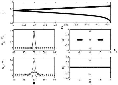
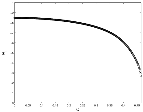
FIG. 2.: The top panel shows the norms $P_{u}$ (lower curve) and $P_{v}$ (upper curve) of the two components of the soliton solution vs. $C$, up to the point where the branch terminates. The next set of panels shows two examples of the solution at $C=0.1$ (the upper row) and $C=0.464$ (just near the termination point of the branch; the lower row), together with the spectral planes of the corresponding linear stability eigenvalues (the vertical and horizontal coordinates in the plane correspond to the imaginary and real parts of $\omega$). The profiles of the $u_{n}$ and $v_{n}$ components are shown, respectively, by circles and stars. These solutions are always unstable. The bottom panel shows the imaginary part of the single unstable eigenfrequency vs. $C$.

An example of the development of the instability of this solution, as found from direct simulations of the full equations (2) and (3), is given in Fig. 3 for $C=0.1$. It is clearly seen that the unstable soliton turns into a stable breather.

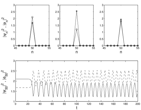
FIG. 3.: Evolution of the unstable soliton from Fig. 2) in the case $C=0.1$, $\beta=0$, and $\kappa=0.1$. The top panel shows the fields’ spatial profiles (the circles correspond to $|\psi_{n}|^{2}$, and the stars to $|\phi_{n}|^{2}$) for $t=4$ (left panel), $t=192$ (middle panel) and $t=196$ (right panel). The first profile is nearly identical to the initial condition, while the other two were chosen close to points where the oscillating amplitude of the resultant breather attains its maximum and minimum. The bottom panel shows the field evolution at the central lattice site ($n=50$), clearly demonstrating the breathing nature of the established state. The solid and dashed lines are, respecively, $|\psi_{50}|^{2}$ and $|\phi_{50}|^{2}$. In this case, the instability growth rate of the initial soliton is $\approx 0.8$; in view of this large value, it was not necessary to add any initial perturbation to trigger the instability.

On the contrary, in the presence of XPM with the physically relevant value of $\beta=2$, a similar solution branch, found for the same values $\kappa=0.1$ and $\Lambda=2$, is stable for all $C$, until it terminates at $C=0.499$. Note that, at this point, the upper edge (10) of the phonon band is $\Lambda_{{\rm edge}}=1.999$, which is extremely close to $\Lambda=2$, i.e., the termination of the solution family is indeed accounted for by its crash into the swelling phonon band. Details of this stable branch are shown in Fig. 4.

Direct simulations of this solution have corroborated its stability (details are not shown here). In fact, in all the cases when solitons are found to be stable in terms of the linearization eigenvalues (see other cases below), direct simulations fully confirm their dynamical stability.

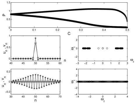
FIG. 4.: The same as in Fig. 2, but for the case $\beta=2$. The middle and lower panels display examples of the soliton solutions at $C=0.1$ and $C=0.499$, respectively. In the top panel, the upper and lower curves now correspond to the $v_{n}$ and $u_{n}$ components, i.e., opposite to the case shown in Fig. 1. Notice that this branch is always stable until it terminates, therefore the figure does not contain a counterpart of the dependence shown in the bottom panel of Fig. 2.

C Solution families which are anti-symmetric in the anti-continuum limit

Another branch of solutions is initiated, in the AC limit, by an anti-symmetric excitation localized at a single lattice site, cf. Eq. (18):

$$u_{n_{0}}=-v_{n_{0}}=\pm\sqrt{\frac{\Lambda+\kappa}{1+\beta}}.$$ (18)

The solution belonging to this branch is shown in Fig. 5 for the same values of parameters as in Fig. 2, i.e., $\delta=1$, $\kappa=0.1$, $\Lambda=2$, and $\beta=0$. With the increase of $C$, this branch picks up an oscillatory instability at $C\approx 0.257$, and terminates at $C\approx 0.407$. Unlike the solutions displayed above, the termination of this branch occurs not through its crash into the phonon band, but via a saddle-node bifurcation. The latter bifurcation implies a collision with another branch of solutions. That additional branch (which is strongly unstable) was found but is not shown here.

In fact, the numerical algorithm is able to capture other solutions (unstable ones) past the point $C\approx 0.407$ at which the present solution terminates. The newly found solutions are shown in the bottom part of Fig. 5. However, the new family cannot be continued beyond $C=0.467$ [cf. the termination point $C=0.464$ for the solutions initiated in the AC limit by the expression (17)].

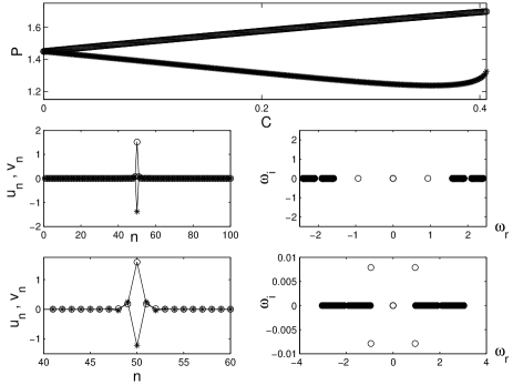
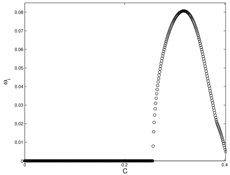
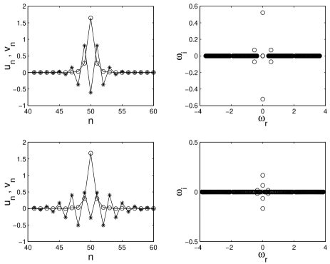
FIG. 5.: The top panel shows the branch of solutions starting from the expression (18) in the AC limit. Two particular examples are shown for $C=0.1$ (a stable solution, the upper row) and $C=0.257$ (at the onset of the oscillatory instability, the lower row). The circles and stars again denote the $u_{n}$ and $v_{n}$ components, respectively. The panel beneath this displays the instability growth rate, ${\rm Im}\,\omega$, vs. $C$. Finally, the bottom panels show the profiles and linear stability eigenvalues for another solution, found beyond the termination point of this branch at $C=0.407$. Two examples of the new solution are given for $C=0.407$ (the upper row) and $C=0.467$ (the lower row). These two points are very close to the beginning and termination of the new branch).

The development of the oscillatory instability of the solution shown in Fig. 5 was also studied in direct simulations. It leads to onset of a state where one component of the soliton is fully destroyed [it cannot completely disappear, due to the presence of the linear couplings in Eqs. (2) and (3), but it is reduced to a level of small random noise]. An example of this is given in Fig. 6 for $C=0.3$, $\beta=0$ and $\kappa=0.1$. The instability (with the initial growth rate $0.07$ in this case) develops after $t\approx 60$, destroying one component of the soliton in favor of further growth of the other one. In this case, a uniformly distributed noise perturbation of an amplitude $10^{-4}$ was added to accelerate the onset of the instability, as the initial instability is very weak (which implies that the unstable soliton may be observed in experiment).

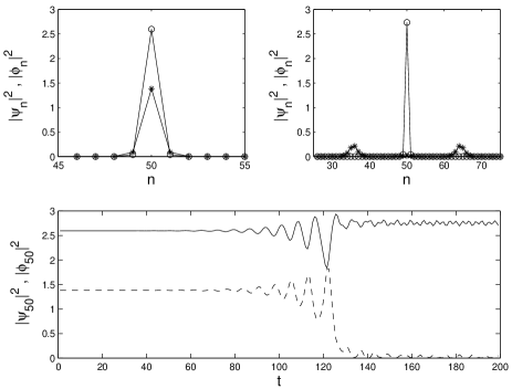
FIG. 6.: Dynamical development of the oscillatory instability of the anti-symmetric solution for $C=0.3$, $\beta=0$ and $\kappa=0.1$. The meaning of the symbols is as in Fig. 3. The top left and right panels show the field configuration at $t=4$ and $t=196$, respectively. The bottom panel once again shows the field evolution at the central site.

A counterpart of the solution from Fig. 5, but with $\beta=2$, rather than $\beta=0$, is shown in Fig. 7. This branch is always unstable (i.e., in the case of the solutions starting from the anti-symmetric expression in the AC limit, the XPM nonlinearity destabilizes the solitons, while in the case of the branch that was initiated by the symmetric expression in the AC limit, the same XPM nonlinearity was stabilizing). It terminates at $C\approx 0.219$, again through a saddle-node bifurcation. As in the previous case, a new family of solutions can be captured by the numerical algorithm past the termination point. The new family is found for $0.22<C<0.498$, and it is also shown in Fig. 7. Comparing the value $\Lambda_{{\rm edge}}=1.995$ given by Eq. (10) in this case with the actual value $\Lambda=2$ of the soliton’s propagation constant, we conclude that the termination of the latter branch is caused by its collision with the phonon band. Notice also that the latter branch becomes unstable only very close to its termination point, at $C>0.494$.

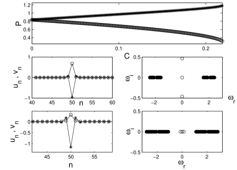
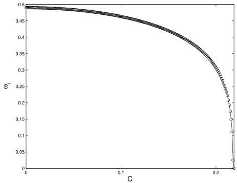
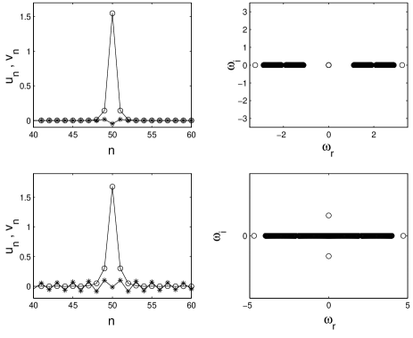
FIG. 7.: The same as in Fig. 5, but for $\beta=2$. This branch is always unstable (as is shown by the middle plot demonstrating the instability growth rate vs. $C$) in its range of existence, $0<C<0.219$. Examples of the solution displayed in the upper part of the figure are given for $C=0.1$ and $C=0.219$. The lower part shows the new solution family found past the termination point of the unstable branch. Example of the new solutions are given for $C=0.22$ (stable, the upper row) and $C=0.498$ (just prior to the termination of the new family, the lower row). The instability of this branch sets in at $C\approx 0.494$, i.e., very close to the termination point.

In the case of $\beta=2$, direct simulations show that the instability of the anti-symmetric branch gives rise to rearrangement of the solution into a very regular breather shown in Fig. 8 for $C=0.1$ and $\kappa=0.1$.

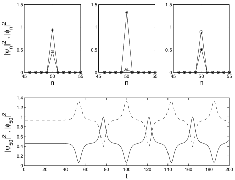
FIG. 8.: The development of the instability accounted for by the imaginary eigenfrequency (with the growth rate $\approx 0.45$) of the anti-symmetric branch, in the case of $C=0.1$, $\kappa=0.1$. The top panels pertain to $t=4$ (left), $t=100$ (middle) and $t=120$ (right). The latter two have again been chosen close to the points where the oscillating amplitude of the resultant breather attains its maximum and minimum, respectively. The instability sets in around $t\approx 40$; no external perturbation was added to the initial condition in this case.

D Solution families which are asymmetric in the anti-continuum limit

Additional branches of the solutions may start in the AC limit from asymmetric configurations, provided that $\Lambda$ is still larger, namely for $\Lambda>2\kappa$. In particular, such an extra branch can be initiated by the following AC-limit solution excited at a single site $n=n_{0}$ (here, $\beta=0$), cf. Eqs. (17) and (18):

$$u_{n_{0}}^{2} = {\frac{1}{2}\left[\Lambda\pm\sqrt{\Lambda^{2}-4\kappa^{2}}\right]},$$ (19)

$$v_{n_{0}} = \kappa^{-1}(\Lambda u_{n_{0}}-u_{n_{0}}^{3})\,.$$ (20)

An example of this solution for the upper sign in Eq. (19) is shown, for $\Lambda=2$, $\kappa=0.5$ and $\delta=1$, in Fig. 9. Such asymmetric branches may be stable for sufficiently weak coupling (in this case, for $C<0.204$), but they eventually become unstable, and disappear soon thereafter (at $C\approx 0.213$, in this case).

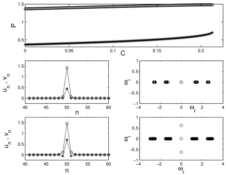
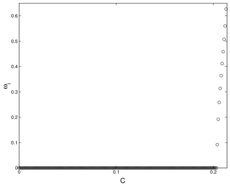
FIG. 9.: The solution branch generated, in the AC limit, by the asymmetric expression (19)-(20) with the upper sign. The notation is the same as in Fig. 2. Two examples of the solution are shown for $C=0.1$ and $C=0.213$. The most unstable eigenvalue is shown, vs. $C$, in the bottom panel. The instability sets in at $C\approx 0.204$, and the branch terminates at $C\approx 0.213$.

The evolution of the instability (for $C>0.204$) for this asymmetric branch is strongly reminiscent of that shown in Fig. 3, resulting in a persistent breathing state.

The branch that commences from the AC expression (19) with the lower sign is shown for $\Lambda=2$, $\kappa=0.75$ and $\delta=1$ in Fig. 10. The branch remains stable as long as it exists, i.e., for $C<0.46$. At this point, it disappears colliding with the phonon band, whose upper edge is located, according to Eq. (10), at $\Lambda_{{\rm edge}}\approx 1.987$, which is very close to the family’s fixed propagation constant, $\Lambda=2$.

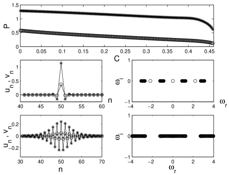
FIG. 10.: The same as in Fig. 9, but generated by the expression (19) with the lower sign. This solution is always stable until it terminates at $C\approx 0.458$. Examples of the solution for $C=0.2$ and $C=0.458$ (the latter case is chosen just prior to the termination of the branch) are shown, as usual, by means of their profiles and linear stability eigenfrequencies.

III Gap solitons

A Solitons in the inner layer of the gap

All the solutions that were examined in the previous section had their propagation constant above the upper edge of the phonon spectrum. Another issue of obvious interest is to study possible gap solitons (GSs), whose propagation constant is located inside the gap (11), i.e., below the lower edge of the phonon band. Unlike the solitons found above the band, GSs may persist up to the continuum limit.

An example of such a solution for $\Lambda=0.75$, $\kappa=-1$, $\delta=0.9$, and $\beta=0$ is shown in Fig. 11. In the AC limit, this branch starts with the expression (17). The branch is stable for small $C$, but then it becomes unstable due to oscillatory instabilities. The first two instabilities occur at $C=0.242$ and $C=0.349$, as is shown in Fig. 11. Past the onset of the instabilities, this branch continues to exist (as an unstable one) indefinitely with the increase of $C$, and carries over into an (unstable) GS in the continuum limit. At large values of $C$, the distinct phonon bands, which are clearly seen in the example of the eigenvalue spectrum shown for $C=0.4$ in Fig. 11, eventually collide and, due to their opposite Krein signs (see the definition and discussion of these in Ref. [16]), which gives rise to a whole set of oscillatory instabilities. The result is clearly seen in the example of the eigenvalue spectrum shown in the bottom panel of Fig. 11 for a large value of the coupling constant, $C=4$. The characteristic size of the instability growth rate (largest imaginary part of the eigenvalue) is nearly the same for $C=0.4$ and $C=4$, in the latter case it being $\approx 0.09$. Notice, however, that, as the continuum limit is approached, the instabilities may be suppressed, in a part or completely, by finite-size effects (for an example of such finite-size restabilization, see Ref. [17]).

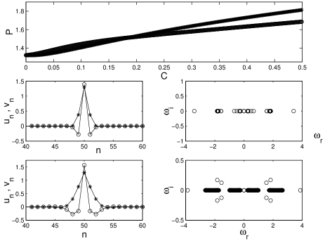
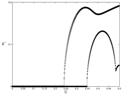
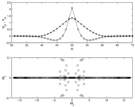
FIG. 11.: The branch of the gap-soliton solutions with $\Lambda=0.75$, $\kappa=-1$, $\delta=0.9$, and $\beta=0$. The upper part of the figure shows the norms of the two components of the soliton, and examples of the solutions for $C=0.1$ (stable) and $C=0.4$ (after the onset of the first oscillatory instability). The middle panel shows the instability growth rates, while the lower part of the figure gives an example of a solution belonging to this branch, found at a much larger value of the coupling constant, $C=4$. This solution family extends, as an unstable one, up to the continuum limit.

The development of the oscillatory instability of GS belonging to the inner layer is displayed, for $C>0.242$, in Fig. 12 for $C=0.4$, $\delta=0.9$, $\kappa=-1$ and $\beta=0$. In this particular case, there are two oscillatory instabilities whose growth rates are in the interval $0.1<\omega_{i}<0.2$. As a result, symmetry breaking occurs, resulting in a shift of the central position of the soliton (from the site $n=50$ to $n=49$). Oscillatory features in the dynamics are also observed in the latter case, and a small amount of energy is emitted as radiation.

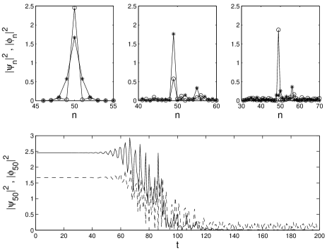
FIG. 12.: The evolution of the unstable gap soliton belonging to the inner layer, for $C=0.4$, $\delta=0.9$, $\kappa=-1$, and $\beta=0$. The top panels shows the wave field distribution at $t=4$ (left), $t=124$ (middle) and $t=132$ (right). Symmetry-breaking effects are clearly visible. A random perturbation of an amplitude $10^{-4}$ was added to the initial condition in order to catalyze the onset of the instability, which occurs at $t>40$.

Similar results were obtained for smaller values of $\Lambda$, for instance, $\Lambda=0.25$. It was verified too that this scenario persists in the presence of the XPM nonlinearity (i.e., for $\beta=2$), as it is shown in Fig. 13. In the latter case, the evolution of the instability with the increase of $C$ is quite interesting, as it is nonmonotonic. The instability first arises at $C\approx 0.11$ (due to a collision between discrete eigenvalues with opposite Krein signs). Subsequent restabilization takes place at $C\approx 0.16$, but the solutions are unstable again for $C>0.36,$ and remain unstable thereafter, up to the continuum limit.

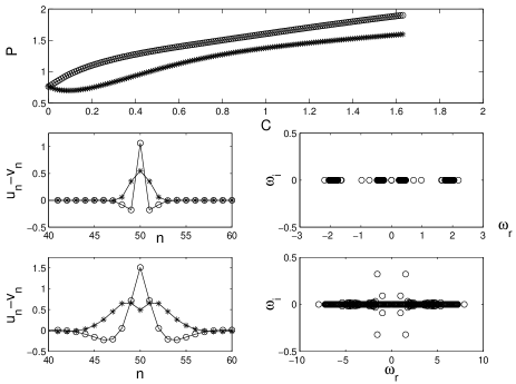
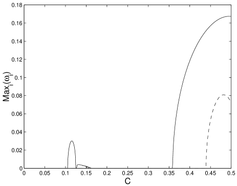
FIG. 13.: The same as the previous figure, but for $\beta=2$. Examples of the solutions are shown for $C=0.2$ (upper row, stable) and $C=1.6$ (lower row, unstable due to several of oscillatory instabilities). The bottom panel demonstrates the nonmonotonic evolution of the instability of this solution with the increase of $C$.

In the case of $\beta=2$, the dynamical development of the oscillatory instabilities is similar to the $\beta=0$ case, again demonstrating symmetry-breaking effects.

B Solutions in the outer layer of the gap

In all the cases considered in the previous subsections, the soliton’s propagation constant $\Lambda$ belonged to the inner layer of the gap, see Eq. (12). We have also examined the situation when $\Lambda$ belongs to the outer layer defined in Eq. (12) (the outer layer exists unless $\delta=1$). An example is shown in Fig. 14, where $\beta=0$, $\kappa=-1$, $\delta=0.1$, and $\Lambda\approx 0.787$ is chosen to be in the middle of the outer layer. In this case, we typically obtained delocalized solitons, sitting on top of a finite background (they are sometimes called “antidark” solitons). As can be observed from Fig. 14, such solutions may be stable for sufficiently weak coupling, but become unstable as the continuum limit is approached, although they do not disappear in this limit (in Ref. [9] such delocalized solitons were found in the continuum counterpart of the present model).

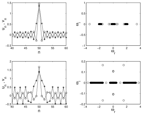
FIG. 14.: Solutions with non-decaying oscillatory background for propagation constants belonging to the outer layer defined by Eq. (12). The top panel shows a stable solution for $C=0.158$, and the bottom panel shows an unstable one of $C=0.576$. These solutions are unstable for all $C>0.341$.

The instability development in the case of the outer-layer GSs is demonstrated, for $C=0.549$, $\beta=0$, $\kappa=-1$ and $\delta=0.1$, in Fig. 15. In this case, the non-vanishing background is also perturbed by the instability, resulting in, plausibly, chaotic oscillations throughout the lattice. Symmetry-breaking effects, which shift the central peak from its original position, are observed too in this case.

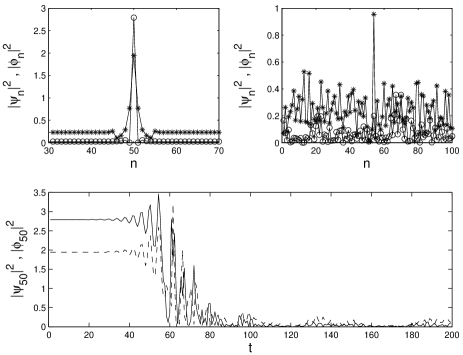
FIG. 15.: The time evolution of the outer-layer gap solitons for $C=0.549$, $\beta=0$, $\kappa=-1$ and $\delta=0.1$. The initial condition is perturbed by a random uniformly distributed perturbation of an amplitude $10^{-4}$. The result of the instability is the excitation of background oscillations, as well as a shift of the soliton’s peak from its original position. The top left and right spatial profiles correspond to $t=4$ and $t=200$, respectively.

C Stabilization of the gap solitons by mismatch

The above considerations show that, inside the inner layer of the gap, it is easy to identify families of soliton solutions that persist in the continuum limit as $C\rightarrow\infty$. However, all the examples considered above showed that the solutions get destabilized at finite $C$ and remain unstable with the subsequent increase of $C$. Therefore, a challenging problem is to find solution families that would remain stable for large values of $C$.

In fact, the introduction of a finite mismatch $q$ (recall it was set equal to zero in all the examples considered above) may easily stabilize the discrete GSs. To this end, we pick up a typical example, with $C=0.5$, $\kappa=-1$, $\delta=0.5$, $\Lambda=0.75$, and $\beta=0$, when the GS exists but is definitely unstable in the absence of the mismatch. Figures 16 and 18 show the effect of positive and negative values of the mismatch on the solitons. As is seen, large values of the positive mismatch can make the instability very weak, but cannot completely eliminate it. However, sufficiently large negative mismatch readily makes the solitons truly stable. Thus, adding the negative mismatch is the simplest way to stabilize the solitons at large $C$, which is not surprising, as Eq. (11) demonstrates that the negative mismatch makes the gap broader.

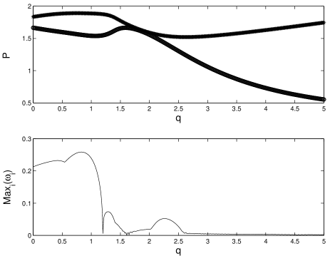
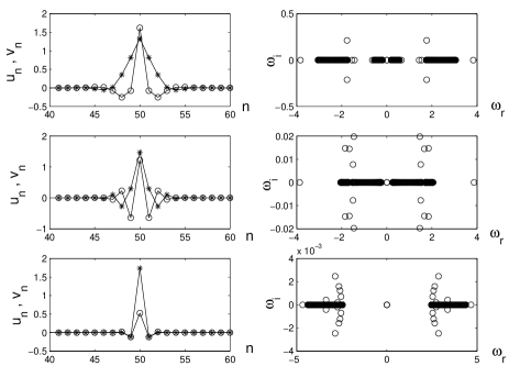
FIG. 16.: A family of the gap-soliton solutions obtained for fixed values $C=0.5$, $\kappa=-1$, $\delta=0.5$, $\Lambda=0.75$, and $\beta=0$, by continuation to positive values of the mismatch parameter $q$. The top panel and the one beneath it show the evolution of the norms of the two components of the solution, and of the largest instability growth rate, with the increase of $q$. Other panels show examples of the solution (as usual, in terms of profiles of the two components and linear stability eigenvalues) for $q=0$, $q=2$, and $q=5$, from top to bottom.

As an example of the dynamical evolution of unstable solitons in the case of positive mismatch, in Fig. 17 we display the case of $C=0.5$, $\kappa=-1$, $\beta=0$, $\delta=0.5$ and $q=1$. In this case, the evolution leads to the establishment of a breather with a rather complex dynamical behavior.

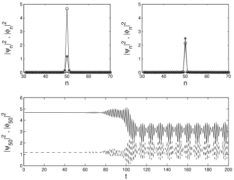
FIG. 17.: The dynamical evolution in the unstable case with $C=0.5$, $\kappa=-1$, $\beta=0$, $\delta=0.5$ and $q=1$ (positive mismatch). The top left and right panels correspond to $t=4$ and $t=396$, respectively. A complex pattern of the amplitude evolution is observed in this case. The initial condition contains a random perturbation with an amplitude $5\times 10^{-5}$.

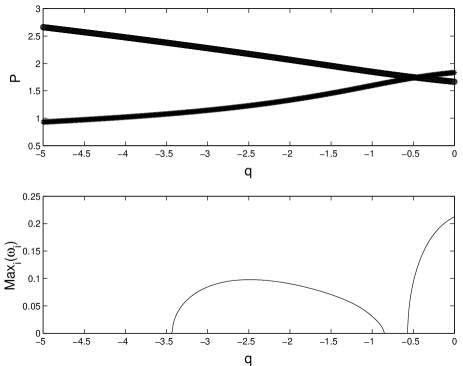
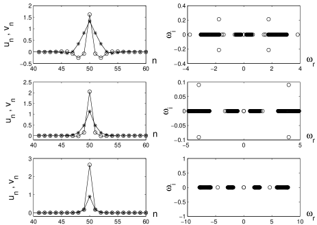
FIG. 18.: The same as in Fig. 16, but for negative values of the mismatch. Examples of the solutions are given for $q=0$, $q=-2$, and $q=-5$, from top to bottom. A random perturbation of an amplitude $10^{-4}$ was used in this case.

The instability development in the case of negative mismatch, $q=-2.5$, is demonstrated in Fig. 19. A localized breather with quasi-periodic intrinsic dynamics is observed in this case as an eventual state.

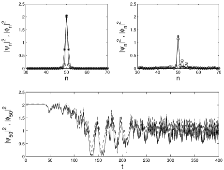
FIG. 19.: The evolution of the unstable discrete gap soliton in with $C=0.5$, $\kappa=-1$, $\beta=0$, $\delta=0.5$ and $q=-2.5$ (negative mismatch). The top left and right panels show the field profiles for $t=4$ and $t=196$, respectively. The time evolution of the amplitudes is shown in the bottom panel.

D Discrete counterparts of gap solitons from the Bragg-grating model

As was shown in the introduction, the particular case of Eqs. (2) and (3) with $\kappa=1$, $\delta=1$, and $\beta=2$ may be interpreted, with regard to the transformation (8), as a discretization of the standard Bragg-grating system (1). This continuum model gives rise to a family of exact GS solutions [19],

$$\Psi=U(x)\,\exp\left(-it\cos\theta\right),\Phi=V(x)\,\exp\left(-it\cos\theta\right),$$ (21)

$$U(x)=\frac{\sin{\rm\,}\theta}{\sqrt{3}}\,{\rm sech}\left(x\sin{\rm\,}\theta-\frac{i}{2}\theta\right),\,V=-U^{\ast},$$ (22)

where the real parameter $\theta$ takes values $0<\theta<\pi$. A part of this interval, $0<\theta<\theta_{{\rm cr}}\approx 1.01\left(\pi/2\right)$, is filled with stable solitons [18], while the remaining part contains unstable ones.

All the discrete GSs considered above are not counterparts of the continuum solitons given by Eqs. (21) and (22). Establishing a direct correspondence between the latter ones and discrete solitons of Eqs. (2) and (3) is complicated by two problems: the transformation (8) does not have a continuum limit, and real symmetric or anti-symmetric GSs with $\left|\Lambda\right|<\kappa$ do not exist in the AC limit, as is seen from Eqs. (17) and (18), i.e., the usual starting point of the analysis is not available in this case.

We have considered the discrete analogs of the Bragg-grating GSs in the following way. First, we took a formal discrete counterpart of the waveforms (21) and (22), and used them to obtain exact solutions of the (formal) discretization of the Bragg-grating model of Eq. (1). Then the transformation (8) was applied to these solutions, and the thus obtained expressions were used as an initial guess for finding a numerically exact stationary solution of Eqs. (2)-(3). This procedure naturally generates new solitons, a crucial difference of which from all the types considered above is that they are truly complex solutions, see examples in Figs. 20 and 21. In this case, we have used $\theta=\pi/4$.

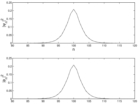
FIG. 20.: Absolute values of the fields in a new complex discrete gap-soliton solution, which was obtained, at $C=1.24$, for the formal discretization of the Bragg-grating gap-soliton model. Then, the transformation (8) was applied to this solution and it was used as an initial condition of the Newton for finding a solution of Eqs. (2)-(3). The continuous and dashed lines (which completely oevrlap) show the resulting profiles generated by the above-mentioned procedure, one which is an exact solution for the discretization of the Bragg-grating model and one which is an exact solution (identical in norm due to the nature of (8)) of Eqs. (2)-(3).

Then, the solution was numerically continued, decreasing $C$, back to the AC limit, in order to identify its AC “stem”. The result is shown in Fig. 21. Obviously, this AC state is very different from all those considered above (in particular, it is complex).

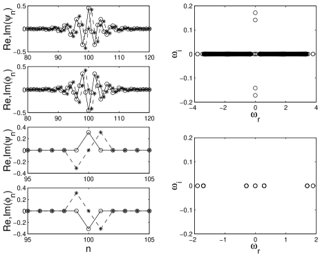
FIG. 21.: Left panels show profiles of real and imaginary parts of the fields $\psi_{n}$ and $\phi_{n}$ in the discrete counterpart of the Bragg-grating gap soliton from Fig. 20. Right panels show stability eigenfrequencies for the same soliton. The upper and lower parts of the figure pertain to the soliton at $C=1.24$ (the same value as in Fig. 20), and to its continuation to the anti-continuum limit, $C=0$. In the left panels, the circles (joined by solid lines) refer to the real parts, while the stars (connected by dashed lines) correspond to the imaginary parts of the corresponding shown fields.

Finally, linear stability eigenvalues were calculated for this new branch of the discrete GSs. The result (see Fig. 22) is that this branch is unstable for all finite values of $C$, getting asymptotically stable in both limits $C\rightarrow 0$ and $C\rightarrow\infty$ (large values of $C$ are not shown in Fig. 22); the stability regained in the latter limit complies with the above-mentioned finding that a subfamily of the continuum Bragg-grating gap solitons are dynamically stable. Notice that the natural norm of the continuum soliton differs from that of the discrete one, given by Eq. (14), by an additional multiplier $C^{-1/2}$ (which is proportional to the effective lattice spacing). We have checked that the thus renormalized norm of the soliton converges as $C\rightarrow\infty$, although data for large $C$ is not displayed in Fig. 22.

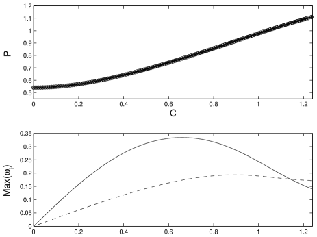
FIG. 22.: The norm of the discrete counterpart of the Bragg-grating gap soliton of the model of Eqs. (2)-(3) (upper panel), and its two unstable (imaginary) eigenfrequencies (lower panel shown by solid and dashed lines respectively), vs. the coupling constant. The continuation of the figure to larger values of $C$ shows that the soliton becomes asymptotically stable as $C\to\infty$.

IV Solitons in the model with the quadratic nonlinearity

Stationary solutions of the SHG system (4) and (5) are looked for in an obvious form, cf. Eqs. (13):

$$\psi_{n}=e^{i\Lambda t}u_{n},\,\phi_{n}=e^{2i\Lambda t}v_{n},$$ (23)

and in this case we only consider the (most characteristic) case $\delta=1$. The linearization of Eqs. (4) and (5) demonstrates that one may expect termination of a soliton-solution branch, due to its collision with the phonon band, at (or close to) the point

$$\Lambda=\kappa/4+C,$$ (24)

and the gap between two phonon bands is

$$0<\Lambda<\kappa/4$$ (25)

(it exists only if $\kappa>0$).

Stationary solutions were constructed, again, by means of continuation starting from the AC limit, where the excitation localized on a single site of the lattice assumes the form

$$v_{n_{0}} = \Lambda,$$ (26)

$$u_{n_{0}} = \pm\sqrt{v_{n_{0}}(4\Lambda-\kappa)}.$$ (27)

Note that solutions with the propagation constant belonging to the gap (25) do not exist close to the AC limit. Indeed, the AC expression (27) shows that a necessary condition for its existence is $4\Lambda>\kappa$. On the other hand, $\Lambda$ stays in the gap (25) if $4\Lambda<\kappa$, so the two conditions are incompatible.

A typical example of a numerically found soliton branch is shown, for the value of the mismatch parameter $\kappa=0.9$, in Fig. 23. This solution family is fixed by choosing $\Lambda=0.25$, and starting from the expressions (26) and (27) with the upper sign. It is seen that the branch is stable for $C<0.015$, but then it becomes unstable, and eventually terminates at $C\approx 0.025$, in very good agreement with the prediction of Eq. (24).

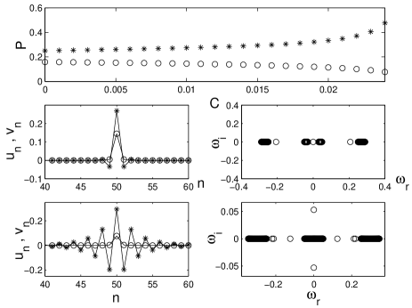
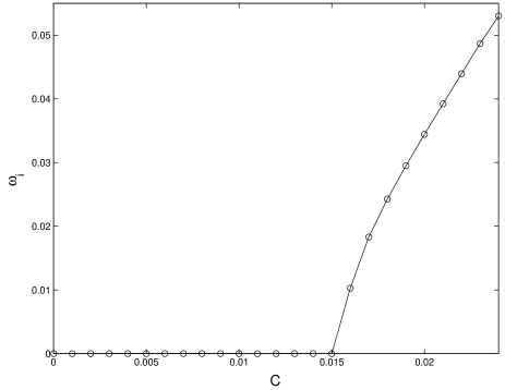
FIG. 23.: The family of the discrete SHG solitons found for $\kappa=0.9$, $\delta=1$, and $\Lambda=0.25$. The top panel shows the evolution of the norms of the fundamental- (circles) and second-frequency (stars) components of the soliton, which are defined the same way as in Eq. (14), with the increase of $C$. Examples of solutions are displayed for $C=0.01$, below the instability threshold, which is $C_{{\rm cr}}=0.015$ (the upper row), and for $C=0.024$, just prior to the termination of the branch at $C=0.025$ (the lower row). The bottom panel shows the evolution of the instability growth rate (imaginary part of the most unstable eigenvalue).

Development of the instability of this SHG soliton branch for $C>0.015$ was numerically examined through direct simulations, results of which are presented in Fig. 24, for the case of $C=0.02$, the corresponding instability growth rate being $\approx 0.03$. A random uniformly distributed perturbation of an amplitude $10^{-4}$ was added to the initial condition to accelerate the onset of the instability. The eventual result of the instability is the appearance of a breather with very regular periodic intrinsic vibrations.

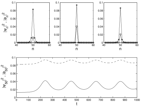
FIG. 24.: Simulations of the instability development for the discrete SHG soliton in the case with $C=0.02$, $\kappa=0.9$ and $\delta=1$. The circles in the spatial profiles of the top panels denote the fundamental, and the stars denote the second harmonic. The left panel corresponds to $t=4$, the middle to $t=660$ (close to the point where the oscillating amplitude attains its maximum), and the right to $760$ (close to a minimum-amplitude point). The bottom panel shows the oscillatory behavior at the central site for the fundamental (solid line) and second harmonics (dashed line).

A similar result for the case without a gap in the phonon spectrum [see Eq. (25)] is shown in Fig. 25 for $\kappa=-0.1$, the other parameters being the same as in the previous case. This time, the branch terminates at $C\approx 0.275$, once again in complete agreement with the prediction of Eq. (24).

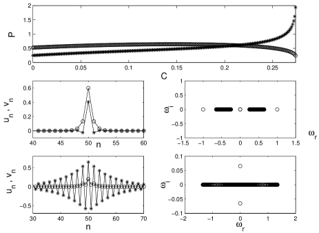
FIG. 25.: The same as in the upper part of Fig. 24, but for $\kappa=-0.1$. The middle panel shows an example of the solution for $C=0.1$, and the bottom panel shows an example for $C=0.274$, just prior to the termination of the branch (which happens at $C=0.275$).

Lastly, another characteristic branch of solutions can be constructed starting from the pattern given by Eqs. (27) with the lower sign. This solution family is displayed in Fig. 26, for $\kappa=0.75$, $\delta=1$, and $\Lambda=0.25$. The branch is stable for sufficiently weak coupling, but then it becomes unstable for $C>0.046$. The branch disappears colliding with the phonon band at $C\approx 0.062$, once again in full agreement with the prediction of Eq. (24).

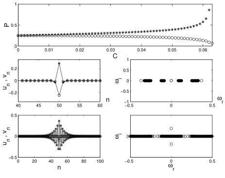
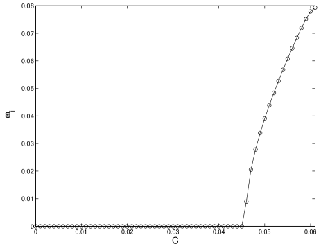
FIG. 26.: The same as in Fig. 23, but for the lower sign in Eq. (27). The middle panel of the top subplot displays an example of a stable solution for $C=0.01$, while the bottom panel shows a solution for $C=0.061$, close to the termination of the branch. In this case, $\kappa=0.75$, $\delta=1$, and $\Lambda=0.25$.

An example of the development of instability of the present solution, that takes place at $C>0.046$, is shown in Fig. 27 for $C=0.055$ ($\kappa=0.75$; $\delta=1$). A random initial perturbation with an amplitude $10^{-4}$ was added to the initial condition in this case. As is seen, the evolution results in complete destruction of the pulse into small-amplitude radiation waves.

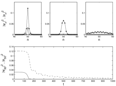
FIG. 27.: The evolution of the unstable SHG soliton in the case of $C=0.055$, $\kappa=0.75$ and $\delta=1$. The top left, middle, and right panels correspond to the profiles at $t=4$, $t=160$, and $t=400$. The bottom panel, as before, shows the time evolution of amplitudes at the central site.

V Conclusion

In this work, we have introduced a model which includes two nonlinear dynamical chains with linear and nonlinear couplings between them, and opposite signs of the discrete diffraction inside the chains. In the case of the cubic nonlinearity, the model finds two distinct interpretations in terms of nonlinear optical waveguide arrays, based on the diffraction-management concept. A continuum limit of the model is tantamount to a dual-core nonlinear optical fiber with opposite signs of dispersion in the two cores. Simultaneously, the system is equivalent to a formal discretization of the standard model of Bragg-grating solitons. A straightforward discrete second-harmonic-generation [$\chi^{(2)}$] model, with opposite signs of the diffractions at the fundamental and second harmonics, was introduced too. Starting from the anti-continuum (AC) limit and gradually increasing the coupling constant, soliton solutions in the $\chi^{(3)}$ model were found, both above the phonon band and inside the gap. Above the gap, the solitons may be stable as long as they exist, but with transition to the continuum limit they inevitably disappear. On the contrary, solitons in the gap persist all the way up to the continuum limit. In the zero-mismatch case, they always become unstable before reaching the continuum limit, but finite mismatch may strongly stabilize them. A separate procedure had to be developed to search for discrete counterparts of the well-known Bragg-grating gap solitons. As a result, it was found that discrete solitons of this type exist at all values of the coupling constant $C$, but they appear to be stable solely in the limit cases $C=0$ and $C=\infty$. Solitons were also found in the $\chi^{(2)}$ model. They too start as stable solutions, but then lose their stability.

In the cases when the solitons were found to be unstable, simulations of their dynamical evolution reveal a variety of different scenarios. These include establishment of localized breathers featuring periodic, quasi-periodic, or very complex intrinsic dynamics, or destruction of one component of the soliton, as well as symmetry-breaking effects, and even complete decay of both components into small-amplitude radiation. The outcome depends on the type of the nonlinearity (cubic or quadratic), and on the nature of the unstable solution.

REFERENCES

- [1] H.S. Eisenberg, Y. Silberberg, R. Morandotti, A. Boyd, and J.S. Aitchison, Phys. Rev. Lett. 81, 3383 (1998); H. S. Eisenberg, R. Morandotti, Y. Silberberg, J. M. Arnold, G. Pennelli, J. S. Aitchison, J. Opt. Soc. Am. B 19, 2938 (2002).
- [2] H.S. Eisenberg, Y. Silberberg, R. Morandotti, A. Boyd, and J.S. Aitchison, Phys. Rev. Lett. 85, 1863 (2000).
- [3] T. Pertsch, T. Zentgraf, U. Peschel, and F. Lederer, Phys. Rev. Lett. 88, 093901 (2002).
- [4] M.J. Ablowitz and Z.H. Musslimani, Phys. Rev. Lett. 87, 254102 (2001).
- [5] U. Peschel and F. Lederer, J. Opt. Soc. Am. B 19, 544 (2002).
- [6] M.J. Ablowitz and Z.H. Musslimani, Phys. Rev. E 65 , 056618 (2002).
- [7] D.N. Christodoulides and R.I. Joseph, Phys. Rev. Lett. 62, 1746 (1989); A.B. Aceves and S. Wabnitz, Phys. Lett. A 141, 37 (1989).
- [8] C.M. de Sterke and J.E. Sipe, Progr. Opt. 33, 203-260 (1994); R. Kashyap, Fiber Bragg gratings (Academic Press: San Diego, 1999).
- [9] D.J. Kaup and B.A. Malomed, J. Opt. Soc. Am. B 15, 2838 (1998).
- [10] J. Hudock, P.G. Kevrekidis, B.A. Malomed, and D.N. Christodoulides, Discrete vector solitons in two-dimensional nonlinear waveguide arrays: solutions, stability and dynamics, submitted to Phys. Rev. E.
- [11] A.A. Sukhorukov and Yu.S. Kivshar, arXiv:nlin.PS/0208036.
- [12] S. Darmanyan, A. Kobyakov and F. Lederer, Phys. Rev. E 57, 2344 (1998); V.M. Agranovich, O.A. Dubovsky, A.M. Kamchatnov, and P. Reineker, Mol. Cryst. Liq. Cryst. 355, 25 (2001); A.A. Sukhorukov, Yu.S. Kivshar, O. Bang and C.M. Soukoulis, Phys. Rev. E 63, 016615 (2001).
- [13] C. Etrich, F. Lederer, B.A. Malomed, T. Peschel, and U. Peschel, Progr. Opt. 41, 483 (2000).
- [14] G.P. Agrawal. Nonlinear Fiber Optics (Academic Press: San Diego, 1995).
- [15] In particular, eigenvalue subroutines implemented within Matlab (see e.g., www.mathworks.com) were used.
- [16] J.-C. van der Meer, Nonlinearity 3, 1041 (1990); S. Aubry, Physica D 103, 201 (1997).
- [17] M. Johansson and Yu.S. Kivshar, Phys. Rev. Lett. 82, 85 (1999).
- [18] B.A. Malomed and R.S. Tasgal, Phys. Rev. E 49, 5787 (1994); I.V. Barashenkov, D.E. Pelinovsky, and E.V. Zemlyanaya, Phys. Rev. Lett. 80, 5117 (1998).
- [19] A.B. Aceves and S. Wabnitz, Phys. Lett. A 141, 37 (1989); D.N. Christodoulides and R.I. Joseph, Phys. Rev. Lett. 62, 1746 (1989).