Feedback Loops Between Fields and Underlying Space Curvature: an Augmented Lagrangian Approach

Abstract

We demonstrate a systematic implementation of coupling between a scalar field and the geometry of the space (curve, surface, etc.) which carries the field. This naturally gives rise to a feedback mechanism between the field and the geometry. We develop a systematic model for the feedback in a general form, inspired by a specific implementation in the context of molecular dynamics (the so-called Rahman-Parrinello molecular dynamics, or RP-MD). We use a generalized Lagrangian that allows for the coupling of the space’s metric tensor (the first fundamental form) to the scalar field, and add terms motivated by RP-MD. We present two implementations of the scheme: one in which the metric is only time-dependent [which gives rise to ordinary differential equation (ODE) for its temporal evolution], and one with spatio-temporal dependence [wherein the metric’s evolution is governed by a partial differential equation (PDE)]. Numerical results are reported for the (1+1)-dimensional model with a nonlinearity of the sine-Gordon type.

Recently, much attention has been focused on soft-condensed-matter objects, such as vesicles, microtubules, and membranes [1, 2, 3, 4]. Many nanoscale physical systems, including nanotubes and electronic and photonic waveguide structures [5, 6], have nontrivial geometry and are influenced by substrate effects. These classes of systems, many of which are inherently nonlinear, raise the question of the interplay between nonlinearity and a substrate with variable curvature. Of particular interest is a possibility of developing curvature in the substrate due to forces generated by the nonlinear field. The resulting curvature can in turn affect the field.

There is an increasing body of literature dealing with the interplay of nonlinearity and a curved substrate. Usually, however, the substrate geometry is assumed to be fixed, see, e.g., [7]. Nevertheless, for many applications, ranging from condensed matter to optics to biophysics, it is relevant to introduce models that admit a flexible substrate, which is affected by the field(s) that it carries, as well as feeding back into the field dynamics. In this situation, equations for the fields in a nonlinear system abutting on the flexible substrate should include both the field dynamics proper and the feedback coupling to the substrate. Equations for the evolution of the substrate should in turn be affected by the evolution of the field. A prototypical physical example of this type is Euler buckling [8], where the evolution of a thermal profile causes the underlying surface to buckle (and hence locally modify its curvature).

In a discrete setting, a model of this type has recently been presented in [9]. However, it was limited to a system of masses coupled by nonlinear springs. Some studies have also been performed in a special case of the continuum limit of classical spin systems (such as the Heisenberg chain) coupled to the curvature; geometric frustration was found to arise in such settings [10].

About twenty years ago, a problem similar to the theme of our study was examined in the context of molecular dynamics studies of structural transitions in crystals. In particular, in a series of papers [11], Rahman and Parrinello introduced a new idea for studying such transitions by means of an augmented Lagrangian that would account for the degrees of freedom of the “box” (the cell) in which the MD particles lie. In studying the time evolution of the box dynamics (naturally obtained through the Euler-Lagrange equations of the augmented Lagrangian for the box degrees of freedom), they were able to identify structural transitions (under external shear) from square to hexagonal patterns, fcc to bcc etc. We will hereafter refer to this technology as the RP-MD method. The relevant Lagrangian for the particles and the box in this case reads:

$$L=\frac{1}{2}\sum_{i}m_{i}{\bf\dot{s}}_{i}G{\bf\dot{s}}_{i}-\sum_{i,j>i}V(r_{ij})+\frac{1}{2}W{\rm Tr}(\dot{f}^{{\rm T}}\dot{f}),$$ (1)

where $m_{i}$ is the mass of the $i$-th particle, ${\bf\dot{s}}_{i}$ is its vectorial velocity, the spatial part $G$ of the spatiotemporal metric tensor may be represented in terms of another matrix $f$ as $G=f^{{\rm T}}f$ ($G$ is positive definite). ^T and ${\rm Tr}$ denote the transposition and trace respectively, $r_{ij}$ and $V$ are distances between the particles and the potential of interaction between them, and $W$ is an effective mass of the box.

Our purpose in this work is to extend the RP-MD methodology to the case of a continuum scalar field, coupled to either a spatially averaged geometric characteristic (“average curvature”), which will give rise to an ODE, or to a spatiotemporal curvature field, that will generate a PDE. The continuum field may represent, e.g., a chemical concentration propagating over a membrane, or a salt solution, causing the swelling of a polymer gel [12], or an envelope wave of the electric field in nanosystems. The spatiotemporal metric is assumed to have the simple form,

$$g=\left(\begin{array}[]{cc}-1&0\\ 0&G\end{array}\right).$$ (2)

We will first consider the general case, where $G$ is a $d\times d$ matrix, $d$ being the space dimension.

One can define a field-type generalization of the RP-MD model, with a scalar field $\phi$, as follows:

$$L=\int d^{d}x\left[-g^{ij}\frac{\partial\phi}{\partial x^{i}}\frac{\partial\phi}{\partial x^{j}}-V(\phi)\right]+\frac{1}{2}W{\rm Tr}(\dot{f}^{{\rm T}}\dot{f}),$$ (3)

where $V(\phi)$ is a potential governing the nonlinear evolution of the field $\phi$ and $f=f(t)$ (only). If $f$ (and hence $G$) is a function of both spatial coordinates and time, an elastic-energy term [13] should be added to the Lagrangian (3), so that it becomes

$\displaystyle L=\int d^{d}x\left[-g^{ij}\frac{\partial\phi}{\partial x^{i}}\frac{\partial\phi}{\partial x^{j}}-V(\phi)\right]+$

$$\int d^{d}x\left\{\frac{1}{2}W\left[{\rm Tr}(\dot{f}^{{\rm T}}\dot{f})-\frac{1}{2}{\rm Tr}(\frac{\partial f^{{\rm T}}}{\partial x_{i}}\frac{\partial f}{\partial x^{i}})\right]\right\}.$$ (4)

An objective of this brief report is to propose two models that include the feedback to the curvature, and, simultaneously, admit as particular solutions the (unperturbed) solutions for the flat (original) metric. In particular, we choose $G=1+f^{2}$ (so that the metric is positive definite and for $f=0$ has as a special case the original Minkowskian metric). Notice a slight deviation in our choice from the RP case of $G=f^{2}$ [14]. Although the formulation of Eqs. (3)-(4) is very general, we hereafter focus on the $d=1$ case that we will examine in more detail.

Assuming initially that $f=f(t)$ only (e.g., including only an effect of the “mean curvature” on the scalar-field dynamics), the Lagrangian (3) becomes

$$L=\frac{1}{2}W\dot{f}^{2}+\int dx\left[\frac{1}{2}\left(\frac{\partial\phi}{\partial t}\right)^{2}-\frac{1+f^{2}}{2}\left(\frac{\partial\phi}{\partial x}\right)^{2}-V(\phi)\right].$$ (5)

Then, the resulting equations of motion (to which we will hereafter refer as model A) are

$$\phi_{tt} = (1+f^{2})\phi_{xx}-\frac{\partial V}{\partial\phi}$$ (6)

$$Wf_{tt} = -f\int\phi_{x}^{2}dx,$$ (7)

where the subscripts stand for the corresponding partial derivatives.

Notice that the function $f$ is directly related to the scalar curvature of the 1-d space. In particular, the Ricci scalar, which is $R=2R_{1212}/det(g)$ [16] in the general case, in the 1-d case is $R=-2\tilde{f}_{tt}/\tilde{f}$, where $\tilde{f}=\sqrt{1+f^{2}}$.

On the other hand, for a metric with both spatial and temporal dependence (e.g., for $f=f(x,t)$), one arrives at the following Lagrangian:

$\displaystyle L=\int dx\left[\frac{1}{2}\left(\frac{\partial\phi}{\partial t}\right)^{2}-\frac{1+f^{2}}{2}\left(\frac{\partial\phi}{\partial x}\right)^{2}-V(\phi)\right]+$

$$\int dx\left[\frac{W}{2}\left(\frac{\partial f}{\partial t}\right)^{2}-\frac{W}{2}\left(\frac{\partial f}{\partial x}\right)^{2}\right].$$ (8)

The ensuing coupled equations for the scalar field and the curvature (to which we will refer as model B) are

$$\phi_{tt} = \left((1+f^{2})\phi_{x}\right)_{x}-\frac{\partial V}{\partial\phi}$$ (9)

$$Wf_{tt} = Wf_{xx}-f\phi_{x}^{2}.$$ (10)

As a particular application of models A and B, we examine the physically ubiquitous sine-Gordon (sG) potential, $V(\phi)=1-\cos(\phi)$ [15]. It is clear that Eqs. (6)-(7) and (9)-(10) have particular solutions with $f=0$, for which the latter equation of each pair is satisfied trivially, while the former reduces exactly to the sG equation. Basic solitary-wave solutions of the sG equation are the topological soliton (kink),

$$\phi_{{\rm k}}(x,t)=4\tan^{-1}\left[\exp\left(\gamma(x-x_{0}-vt)\right)\right],$$ (11)

where $v$ is its velocity, $\gamma=(1-v^{2})^{-1/2}$ is the Lorentz factor, and $x_{0}$ is the initial position of the kink’s center, and the breather, $\phi_{{\rm br}}(x,t)=4\tan^{-1}\{\sqrt{(1-\omega^{2})/\omega^{2}}\sin\left[\omega\gamma(t-v(x-x_{0}))\right]\times\\ {\rm sech}\left[\gamma\sqrt{1-\omega^{2}}(x-x_{0}-vt)\right]\}$, where $\omega$ is the frequency of its internal oscillations ($0<\omega<1$).

The results of the interaction of the kink with the curvature in model A are shown in Fig. 1 [17]. The curvature variable $f$, initialized with a small random value, performs smooth oscillations with a frequency of $\omega\approx 2.866$. Notice that this is natural in this case, since the kink has an approximately fixed “mass”, $M_{k}=\int_{-\infty}^{+\infty}u_{x}^{2}dx$, which can be found to be $M_{k}=8.247$ for the velocity $v\approx 0.25$). Then, Eq. (7) predicts the frequency of these oscillations $\omega\approx\sqrt{M_{k}}=2.871$, which is very close to the above-mentioned numerically exact value. Fast small-amplitude oscillations of the kink’s velocity, observed in Fig. 1 both with and without the curvature, are due to “hopping” over sites of a lattice (with spacing $h=0.1$) employed in the numerical scheme which solves Eq. (7). Notice, however, that in the top panel the mean velocity is $\approx 0.2503$, while in the bottom panel it is $\approx 0.2499$, hence the curvature oscillations increase the kink’s velocity. This may be anticipated due to the presence of the positive definite factor $1+f^{2}$ in front of $\phi_{xx}$ in Eq. (6), which is expected to renormalize $v^{2}$.

The curvature-breather interaction in model A is shown in Fig. 2. The frequency of the breather does not change significantly (it fluctuates between $0.87$ and $0.93$), but its amplitude decreases substantially (by more than $50\%$), resulting in its becoming much more mobile (the velocity increases to $\approx 0.425$ from the initial value $0.25$).

In model B, we examine collision of a kink with a localized pulse of the substrate field $f$. For the breather, we have obtained results which are qualitatively similar to those presented below for the kink. We create the curvature pulse to the left or to the right of the kink. As $\phi_{x}$ vanishes far from the kink, the equation (10) for $f$ becomes a linear wave equation. Hence, we observe splitting of the pulse into left- and one right-traveling ones. In the case where the kink is initially to the left of the pulse, it collides with the left-propagating fragment of the (split) pulse. In the opposite case, the kink is eventually caught by the co-propagating right fragment of the (split) pulse. Numerical simulations shown in Fig. 3 demonstrate that the collision with the counter-propagating pulse reduces the kink’s velocity, while the interaction with the co-propagating pulse gives rise to an increase of the velocity. In particular, in the former case, the mean speed of the kink after the collision is $\approx 0.2476$, while in the latter one, it increases to $\approx 0.2527$. Notice that in both cases a small fragment of the pulse that collides with the kink passes through it, while a larger fraction of the pulse is reflected by it. The latter feature may be explained by a momentum-balance analysis.

In conclusion, we have extended field theory in the spirit of the Rahman-Parrinello Molecular Dynamics technique. The resulting equations couple the spatio-temporal evolution of the field to that of the underlying curvature of the space which carries the field. Coupled equations for the temporal or spatiotemporal evolution of the metric are obtained in a general setting, and, as an example, are solved together with the sine-Gordon field equation. The purely temporal evolution of the metric has been found to increase the velocity of the field solitons, while the model allowing spatio-temporal evolution of the metric can induce both increase and decrease of the velocity.

It would be particularly interesting to extend the models A and B to higher dimensions. It is also worth studying how the local evolution of the curvature affects kinematics and dynamics of the solitons, and to correlate such observations with the behavior of reactant chemical concentrations in chemical or biological environments with non-trivial geometry [18].

Acknowledgements: The authors acknowledge D. Maroudas for stimulating discussions. The support of NSF and AFOSR (IGK) and NSF (DMS-0204585), UMass and the Clay Institute (PGK) is gratefully acknowledged. Work at Los Alamos is supported by the US DoE.

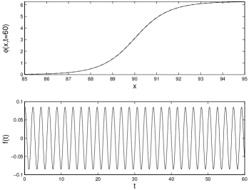
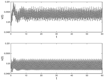
FIG. 1.: The top left panel shows the kink’s spatial profile at $t=60$ in model A. The initial kink profile (centered around the new center position) is shown by the dashed line, and is practically indistinguishable from the solution at $t=60$, indicating that the kink maintains its shape. The bottom left panel shows smooth oscillations of $f(t)$. The top and bottom right panels show, respectively, the kink’s velocity $v(t)$ vs. $t$, and the same quantity but for $f=0$.

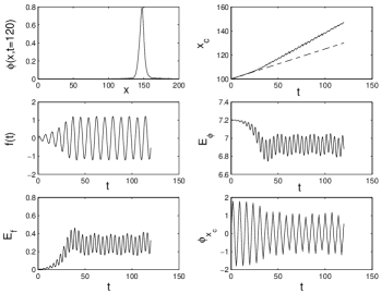
FIG. 2.: The top left and right panels show, respectively, the breather in model A at the end of the simulation period, $t=120$, and its position vs. time (solid), as compared to that which it would have moving at the initial velocity, $v=0.25$ (dashed). The middle left panel shows the time evolution of $f(t)$, while the middle right and bottom left panels present exchange between the curvature-mode’s energy, $E_{f}=f_{t}^{2}/2+(f^{2}/4)\int\phi_{x}^{2}dx$, and the rest of the energy, $E_{\phi}=E-E_{f}$. Finally, the bottom right panel shows the time evolution of the field $\phi$ at the center of the breather.

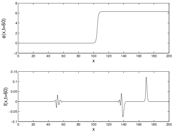
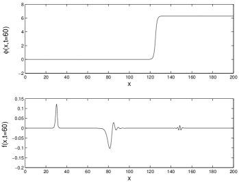
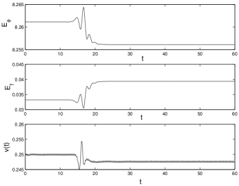
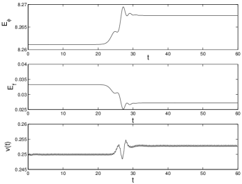
FIG. 3.: The left part of the figure shows spatial profiles of the fields $\phi$ and $f$ at $t=60$ in model B. It also shows the time evolution of the energies $E_{\phi}=E-E_{f}$ and $E_{f}=\int(1/2)(f_{t}^{2}+f_{x}^{2}+(f\phi_{x})^{2}/2)dx$, as well as the kink’s velocity as a function of time. The kink’s center is initially at $x=90$, while the center of the curvature pulse is at $x=110$. The right subplots show counterparts of those in the left part, but for the case of the kink and curvature pulse initially centered at $x=110$ and $x=90$, respectively.

REFERENCES

- [1] E. Sackmann, in R. Lipowsky and E. Sackmann (Eds.), The Structure and Dynamics of Membranes: Handbook of Biological Physics, vol. 1 (Elsevier, Amsterdam, 1995).
- [2] U. Seifert, Adv. in Phys. 46, 13 (1997).
- [3] W. Saenger. Principles of Nucleic Acid Structure (Springer-Verlag: Berlin, 1984).
- [4] J. Meunier, D. Langevin, and D. Boccara (Eds.), Physics of Amphiphilic Layers, Springer-Verlag (Berlin, 1997).
- [5] Y. Imry. Introduction to Mesoscopic Physics (Oxford University Press: New York, 1997).
- [6] C.M. Soukoulis (Ed.), Photonic Band Gaps and Localization, Plenum Press (New York, 1993).
- [7] See e.g., Yu. B. Gaididei, S. F. Mingaleev, and P. L. Christiansen, Phys. Rev. E 62, R53 (2000); M. Ibanes, J. M. Sancho, and G. P. Tsironis, Phys. Rev. E 65, 041902 (2002);
- [8] S.P. Timoshenko and S. Woinowsky-Krieger, Theory of plates and shells, McGraw-Hill (New York, 1959) S.S. Antman, Nonlinear problems of elasticity, Springer-Verlag (New York 1995).
- [9] P.G. Kevrekidis, B.A. Malomed and A.R. Bishop, Phys. Rev. E 66, 046621 (2002).
- [10] S. Villain-Guillot, R. Dandoloff, A. Saxena and A.R. Bishop, Phys. Rev. B 52, 6712 (1995); R. Dandoloff, S. Villain-Guillot, A. Saxena and A.R. Bishop, Phys. Rev. Lett. 74, 813 (1995).
- [11] see e.g., M. Parrinello and A. Rahman, Phys. Rev. Lett. 45, 1196 (1980). M. Parrinello and A. Rahman, J. Appl. Phys. 52, 7182 (1981).
- [12] E. C. Achilleos, R. K. Prud’homme, I. G. Kevrekidis, K. N. Christodoulou and K.R. Gee, AIChE Journal, 46, 2128 (2000).
- [13] Elastic dynamics is a natural first approximation, even though it is possible for the substrate to have more complicated dynamical evolution laws (which can also be incorporated in this setting).
- [14] We also ran detailed simulations of the case with . Here, the non-existence of the original steady state of the field and its competition with the oscillatory behavior of around yields rather unphysical behavior involving large gradients of the field. For these reasons, this case is not presented in detail here.
- [15] R. K. Dodd, J. C. Eilbeck, J. D. Gibbon, and H. C. Morris, Solitons and Nonlinear Wave Equations (Academic Press, London, 1982).
- [16] B. O’Neill, Semi-Riemannian Geometry with Applications to Relativity (Academic Press, London, 1983).
- [17] In the numerical computations has been fixed to . By varying , we have found, similarly to the original works of RP, that its increase slows down the rate at which the presented phenomenology occurs.
- [18] J. Wolff, A.G. Papathanasiou, I.G. Kevrekidis, H.H. Rotermund, and G. Ertl, Science 294, 134 (2001).