PHYSICS Version of
  
Random Noise and Pole-Dynamics in Unstable Front Propagation(new version)

Abstract

The problem of flame propagation is studied as an example of unstable fronts that wrinkle on many scales. The analytic tool of pole expansion in the complex plane is employed to address the interaction of the unstable growth process with random initial conditions and perturbations. We argue that the effect of random noise is immense and that it can never be neglected in sufficiently large systems. We present simulations that lead to scaling laws for the velocity and acceleration of the front as a function of the system size and the level of noise, and analytic arguments that explain these results in terms of the noisy pole dynamics.

I Introduction

In our last paper about flame front propagation we left two open problems. The first one is how to explain the existence of small dependence parameters of problem on the noise. The second problem is how to calculate numerically such values as excess number of poles in system , number of poles that appear in the system in unit of time, life time of pole.To solve these problem we write this paper.

II Equations of Motion and Pole-decomposition in the Channel Geometry

It is known that planar flames freely propagating through initially motionless homogeneous combustible mixtures are intrinsically unstable. It was reported that such flames develop characteristic structures which include cusps, and that under usual experimental conditions the flame front accelerates as time goes on. A model in $1+1$ dimensions that pertains to the propagation of flame fronts in channels of width $\tilde{L}$ was proposed in [4]. It is written in terms of position $h(x,t)$ of the flame front above the $x$-axis. After appropriate rescalings it takes the form:

$${\partial h(x,t)\over\partial t}={1\over 2}\left[{\partial h(x,t)\over\partial x}\right]^{2}+\nu{\partial^{2}h(x,t)\over\partial x^{2}}+I\{h(x,t)\}+1\ .$$ (1)

The domain is $0<x<\tilde{L}$, $\nu$ is a parameter and we use periodic boundary conditions. The functional $I[h(x,t)]$ is the Hilbert transform of derivative which is conveniently defined in terms of the spatial Fourier transform

$$h(x,t)=\int_{-\infty}^{\infty}e^{ikx}\hat{h}(k,t)dk$$ (2)

$$I[h(k,t)]=|k|\hat{h}(k,t)$$ (3)

For the purpose of introducing the pole-decomposition it is convenient to rescale the domain to $0<\theta<2\pi$. Performing this rescaling and denoting the resulting quantities with the same notation we have

$${\partial h(\theta,t)\over\partial t}={1\over 2L^{2}}\left[{\partial h(\theta,t)\over\partial\theta}\right]^{2}+{\nu\over L^{2}}{\partial^{2}h(\theta,t)\over\partial\theta^{2}}$$ (4)

$$+{1\over L}I\{h(\theta,t)\}+1\ .$$ (5)

In this equation $L=\tilde{L}/2\pi$. Next we change variables to $u(\theta,t)\equiv{\partial h(\theta,t)/\partial\theta}$. We find

$${\partial u(\theta,t)\over\partial t}={u(\theta,t)\over L^{2}}{\partial u(\theta,t)\over\partial\theta}+{\nu\over L^{2}}{\partial^{2}u(\theta,t)\over\partial\theta^{2}}+{1\over L}I\{u(\theta,t)\}\ .$$ (6)

It is well known that the flat front solution of this equation is linearly unstable. The linear spectrum in $k$-representation is

$$\omega_{k}=|k|/L-\nu k^{2}/L^{2}\ .$$ (7)

There exists a typical scale $k_{max}$ which is the last unstable mode

$$k_{max}={L\over\nu}\ .$$ (8)

Nonlinear effects stabilize a new steady-state which is discussed next.

The outstanding feature of the solutions of this equation is the appearance of cusp-like structures in the developing fronts. Therefore a representation in terms of Fourier modes is very inefficient. Rather, it appears very worthwhile to represent such solutions in terms of sums of functions of poles in the complex plane. It will be shown below that the position of the cusp along the front is determined by the real coordinate of the pole, whereas the height of the cusp is in correspondence with the imaginary coordinate. Moreover, it will be seen that the dynamics of the developing front can be usefully described in terms of the dynamics of the poles. Following [8, 9, 11, 7] we expand the solutions $u(\theta,t)$ in functions that depend on $N$ poles whose position $z_{j}(t)\equiv x_{j}(t)+iy_{j}(t)$ in the complex plane is time dependent:

$$u(\theta,t)=\nu\sum_{j=1}^{N}\cot\left[{\theta-z_{j}(t)\over 2}\right]+c.c.$$ (9)

$$=\nu\sum_{j=1}^{N}{2\sin[\theta-x_{j}(t)]\over\cosh[y_{j}(t)]-\cos[\theta-x_{j}(t)]}\ ,$$ (10)

$$h(\theta,t)=2\nu\sum_{j=1}^{N}{\ln\Big{[}\cosh(y_{j}(t))-\cos(\theta-x_{j}(t))\Big{]}}+C(t)\ .$$ (11)

In (11) $C(t)$ is a function of time. The function (11) is a superposition of quasi-cusps (i.e. cusps that are rounded at the tip). The real part of the pole position (i.e. $x_{j}$) is the coordinate (in the domain $[0,2\pi]$) of the maximum of the quasi-cusp, and the imaginary part of the pole position (i.e $y_{j}$) is related to the depth of the quasi-cusp. As $y_{j}$ decreases the depth of the cusp increases. As $y_{j}\to 0$ the depth diverges to infinity. Conversely, when $y_{j}\to\infty$ the depth decreases to zero.

The main advantage of this representation is that the propagation and wrinkling of the front can be described via the dynamics of the poles. Substituting (10) in (6) we derive the following ordinary differential equations for the positions of the poles:

$$-L^{2}{dz_{j}\over dt}=\Big{[}\nu\sum_{k=1,k\neq j}^{2N}\cot\left({z_{j}-z_{k}\over 2}\right)+i{L\over 2}sign[Im(z_{j})]\Big{]}.$$ (12)

We note that in (10), due to the complex conjugation, we have $2N$ poles which are arranged in pairs such that for $j<N$ $z_{j+N}=\bar{z}_{j}$. In the second sum in (10) each pair of poles contributed one term. In Eq.(12) we again employ $2N$ poles since all of them interact. We can write the pole dynamics in terms of the real and imaginary parts $x_{j}$ and $y_{j}$. Because of the arrangement in pairs it is sufficient to write the equation for either $y_{j}>0$ or for $y_{j}<0$. We opt for the first. The equations for the positions of the poles read

$$-L^{2}{dx_{j}\over dt}=\nu\sum_{k=1,k\neq j}^{N}\sin(x_{j}-x_{k})\Bigg{[}[\cosh(y_{j}-y_{k})$$ (13)

$$-\cos(x_{j}-x_{k})]^{-1}+[\cosh(y_{j}+y_{k})-\cos(x_{j}-x_{k})]^{-1}\Bigg{]}$$ (14)

$$L^{2}{dy_{j}\over dt}=\nu\sum_{k=1,k\neq j}^{N}\Big{(}{\sinh(y_{j}-y_{k})\over\cosh(y_{j}-y_{k})-\cos(x_{j}-x_{k})}$$ (15)

$$+{\sinh(y_{j}+y_{k})\over\cosh(y_{j}+y_{k})-\cos(x_{j}-x_{k})}\Big{)}+\nu\coth(y_{j})-L.$$ (16)

We note that if the initial conditions of the differential equation (6) are expandable in a finite number of poles, these equations of motion preserve this number as a function of time. On the other hand, this may be an unstable situation for the partial differential equation, and noise can change the number of poles. This issue will be examined at length in Section III. We turn now to a discussion of the steady state solution of the equations of the pole-dynamics.

A Qualitative properties of the stationary solution

The steady-state solution of the flame front propagating in channels of width $2\pi$ was presented in Ref.[9]. Using these results we can immediately translate the discussion to a channel of width $L$. The main results are summarized as follows:

1. There is only one stable stationary solution which is geometrically represented by a giant cusp (or equivalently one finger) and analytically by $N(L)$ poles which are aligned on one line parallel to the imaginary axis. The existence of this solution is made clearer with the following remarks.

2. There exists an attraction between the poles along the real line. This is obvious from Eq.(13) in which the sign of $dx_{j}/dt$ is always determined by $\sin(x_{j}-x_{k})$. The resulting dynamics merges all the $x$ positions of poles whose $y$-position remains finite.

3. The $y$ positions are distinct, and the poles are aligned above each others in positions $y_{j-1}<y_{j}<y_{j+1}$ with the maximal being $y_{N(L)}$. This can be understood from Eq.(16) in which the interaction is seen to be repulsive at short ranges, but changes sign at longer ranges.

4. If one adds an additional pole to such a solution, this pole (or another) will be pushed to infinity along the imaginary axis. If the system has less than $N(L)$ poles it is unstable to the addition of poles, and any noise will drive the system towards this unique state. The number $N(L)$ is

   $$N(L)=\Big{[}{1\over 2}\left({L\over\nu}+1\right)\Big{]}\ ,$$ (17)

   where $\Big{[}\dots\Big{]}$ is the integer part. To see this consider a system with $N$ poles and such that all the values of $y_{j}$ satisfy the condition $0<y_{j}<y_{max}$. Add now one additional pole whose coordinates are $z_{a}\equiv(x_{a},y_{a})$ with $y_{a}\gg y_{max}$. From the equation of motion for $y_{a}$, (16) we see that the terms in the sum are all of the order of unity as is also the $\cot(y_{a})$ term. Thus the equation of motion of $y_{a}$ is approximately

   $${dy_{a}\over dt}\approx\nu{2N+1\over L^{2}}-{1\over L}\ .$$ (18)

   The fate of this pole depends on the number of other poles. If $N$ is too large the pole will run to infinity, whereas if $N$ is small the pole will be attracted towards the real axis. The condition for moving away to infinity is that $N>N(L)$ where $N(L)$ is given by (17). On the other hand the $y$ coordinate of the poles cannot hit zero. Zero is a repulsive line, and poles are pushed away from zero with infinite velocity. To see this consider a pole whose $y_{j}$ approaches zero. For any finite $L$ the term $\coth(y_{j})$ grows unboundedly whereas all the other terms in Eq.(16) remain bounded.

5. The height of the cusp is proportional to $L$. The distribution of positions of the poles along the line of constant $x$ was worked out in [9].

We will refer to the solution with all these properties as the Thual-Frisch-Henon (TFH)-cusp solution.

III Acceleration of the Flame Front, Pole Dynamics and Noise

A major motivation of this Section is the observation that in radial geometry the same equation of motion shows an acceleration of the flame front. The aim of this section is to argue that this phenomenon is caused by the noisy generation of new poles. Moreover, it is our contention that a great deal can be learned about the acceleration in radial geometry by considering the effect of noise in channel growth. In Ref. [9] it was shown that any initial condition which is represented in poles goes to a unique stationary state which is the giant cusp which propagates with a constant velocity $v=1/2$ up to small $1/L$ corrections. In light of our discussion of the last section we expect that any smooth enough initial condition will go to the same stationary state. Thus if there is no noise in the dynamics of a finite channel, no acceleration of the flame front is possible. What happens if we add noise to the system?

For concreteness we introduce an additive white-noise term $\eta(\theta,t)$to the equation of motion (6) where

$$\eta(\theta,t)=\sum_{k}{\eta_{k}(t)\exp{(ik\theta)}}\ ,$$ (19)

and the Fourier amplitudes $\eta_{k}$ are correlated according to

$$<\eta_{k}(t)\eta^{*}_{k^{\prime}}(t^{\prime})>={f\over L}\delta_{k,k^{\prime}}\delta(t-t^{\prime})\ .$$ (20)

We will first examine the result of numerical simulations of noise-driven dynamics, and later return to the theoretical analysis.

A Noisy Simulations

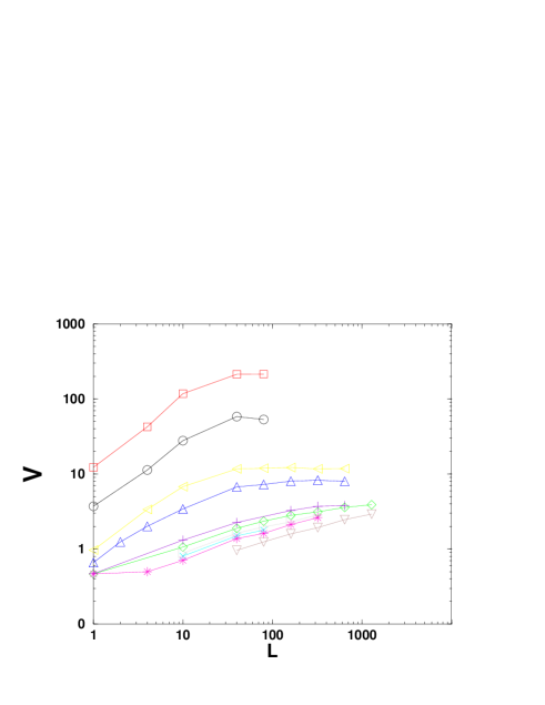
FIG. 1.: The dependence of the average velocity $v$ on the system size $L$ for $f^{0.5}=0,2.7e-6,2.7e-5,2.7e-4,2.7e-3,2.7e-2,2.7e-1,0.5,1.3,2.7$.

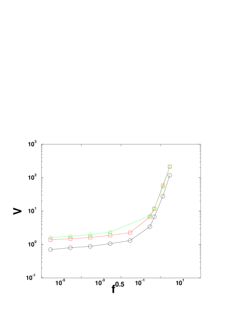
FIG. 2.: The dependence of the average velocity $v$ on the noise $f^{0.5}$ for L=10, 40, 80.

Previous numerical investigations [6, 15] did not introduce noise in a controlled fashion. We will argue later that some of the phenomena encountered in these simulations can be ascribed to the (uncontrolled) numerical noise. We performed numerical simulations of Eq.(6 using a pseudo-spectral method. The time-stepping scheme was chosen as Adams-Bashforth with 2nd order presicion in time. The additive white noise was generated in Fourier-space by choosing $\eta_{k}$ for every $k$ from a flat distribution in the interval $[-\sqrt{2{f\over L}},\sqrt{2{f\over L}}]$. We examined the average steady state velocity of the front as a function of $L$ for fixed $f$ and as a function of $f$ for fixed $L$. We found the interesting phenomena that are summarized here:

1. In Fig.2 we can see two different regimes of behavior the average velocity $v$ as function of noise $f^{0}.5$ for fixed system size L. For the noise $f$ smaller then same fixed value $f_{cr}$

   $$v\sim f^{\xi}\ .$$ (21)

   For these values of $f$ this dependence is very weak, and $\xi\approx 0.02$. For large values of $f$ the dependence is much stronger

2. In Fig.1 we can see growth of the average velocity $v$ as function of the system size L. After some values of L we can see saturation of the velocity. For regime $f<f_{cr}$ the growth of the velocity can be written as

   $$v\sim L^{\mu},\quad\mu\approx 0.40\pm 0.05\ .$$ (22)

B Calculation of Poles Number in the System

The interesting problem that we would like to solve here it is to find number of poles that exist in our system outside the giant cusp. We can make it by next way: to calculate number of cusps (points of minimum or inflexional points) and their position on the interval $\theta:[0,2\pi]$ in every moment of time and to draw positions of cusp like function of time, see Fig.3.

FIG. 3.: The dependence of the cusps positions on time.$L=80$ $\nu=0.1$ $f=9e-6$

We assume that our system is almost all time in ”quasi-stable” state, i.e. every new cusp that appears in the system includes only one pole. By help pictures obtained by such way we can find

1. By calculation number of cusp in some moment of time and by investigation of history of every cusp (except the giant cusp) , i.e. how many initial cusps take part in formation this cusp, after averaging with respect to different moments of time we can find mean number of poles that exist in our system outside the giant cusp. Let us denote this number $\delta N$. We can see four regimes that can be define with respect to dependence of this number on noise $f$:

   (i) Regime I: Such small noise that no poles exist in our system outside the giant cusp.

   (ii) Regime II Strong dependence of poles number $\delta N$ on noise $f$.

   (iii) Regime III Saturation poles number $\delta N$ on noise $f$, so we see very small dependence of this number on noise

   $$\delta N\sim f^{0.03}$$ (23)

   

   FIG. 4.: The dependence of poles number in time unit $dN/dt$ on the noise $f^{0.5}$. $\nu=0.1$ $L=80$

   

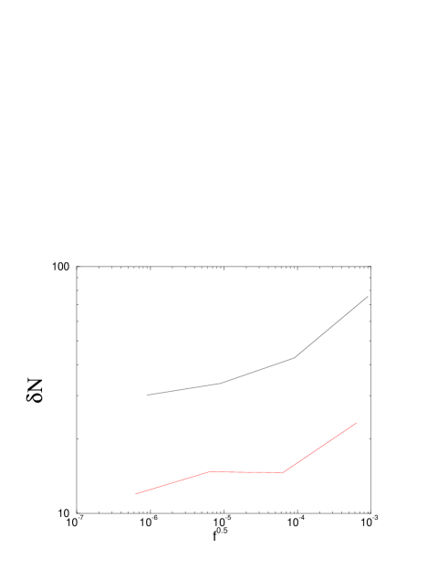
   FIG. 5.: The dependence of excess poles number $\delta N$ on the noise $f^{0.5}$. $\nu=0.1$ $L=40,80$.

   

   FIG. 6.: The dependence of poles number in time unit $dN/dt$ on the system size L. $\nu=0.1$ $f^{0.5}=9e-6$.

   

   FIG. 7.: The dependence of excess poles number $\delta N$ on the system size L. $\nu=0.1$ $f^{0.5}=9e-6$

   

   FIG. 8.: The dependence of poles number in time unit $dN/dt$ on the parameter $\nu$. $L=80$ $\nu=0.1$.

   

   FIG. 9.: The dependence of excess poles number $\delta N$ on the the parameter $\nu$. $L=80$ $\nu=0.1$.

   Saturated value of $\delta N$ is defined by next formula

   $$\delta N\approx N(L)/2\approx{1\over 4}{L\over\nu}$$ (24)

   where $N(L)\approx{1\over 2}{L\over\nu}$ is number of poles in giant cusp.

   (iv) Regime IV We again see strong dependence of poles number $\delta N$ on noise $f$.

   $$\delta N\sim f^{0.1}$$ (25)

   Because of numerical noise we can see in most of simulations only regime III and IV. In future if we don’t note something different we discuss regime III.

2. By calculation of new cusp number we can find number of poles that appear in the system in unit of time ${dN\over dt}$. In regime III

   $${dN\over dt}\sim f^{0.03}$$ (26)

   Dependence on $L$ and $\nu$ define by

   $${dN\over dt}\sim L^{0.8}$$ (27)

   $${dN\over dt}\sim{1\over\nu^{2}}$$ (28)

   And in regime IV

   $${dN\over dt}\sim f^{0.1}$$ (29)

C Theoretical Discussion of the Effect of Noise

1 The Threshold of Instability to Added Noise. Transition from regime I to regime II

First we present the theoretical arguments that explain the sensitivity of the giant cusp solution to the effect of added noise. This sensitivity increases dramatically with increasing the system size $L$. To see this we use again the relationship between the linear stability analysis and the pole dynamics.

Our additive noise introduces perturbations with all $k$-vectors. We showed previously that the most unstable mode is the $k=1$ component $A_{1}\sin(\theta)$. Thus the most effective noisy perturbation is $\eta_{1}\sin(\theta)$ which can potentially lead to a growth of the most unstable mode. Whether or not this mode will grow depends on the amplitude of the noise. To see this clearly we return to the pole description. For small values of the amplitude $A_{1}$ we represent $A_{1}\sin(\theta)$ as a single pole solution of the functional form $\nu e^{-y}\sin{\theta}$. The $y$ position is determined from $y=-\log{|A_{1}|/\nu}$, and the $\theta$-position is $\theta=\pi$ for positive $A_{1}$ and $\theta=0$ for negative $A_{1}$. From the analysis of Section III we know that for very small $A_{1}$ the fate of the pole is to be pushed to infinity, independently of its $\theta$ position; the dynamics is symmetric in $A_{1}\to-A_{1}$ when $y$ is large enough. On the other hand when the value of $A_{1}$ increases the symmetry is broken and the $\theta$ position and the sign of $A_{1}$ become very important. If $A_{1}>0$ there is a threshold value of $y$ below which the pole is attracted down. On the other hand if $A_{1}<0$, and $\theta=0$ the repulsion from the poles of the giant cusp grows with decreasing $y$. We thus understand that qualitatively speaking the dynamics of $A_{1}$ is characterized by an asymmetric “potential” according to

$$\dot{A}_{1} = -{\partial V(A_{1})\over\partial A_{1}}\ ,$$ (30)

$$V(A_{1}) = \lambda A_{1}^{2}-aA_{1}^{3}+\dots\ .$$ (31)

¿From the linear stability analysis we know that $\lambda\approx\nu/L^{2}$, cf. Eq.(18). We know further that the threshold for nonlinear instability is at $A_{1}\approx\nu^{3}/L^{2}$, cf. Eq(LABEL:nu3L2). This determines that value of the coefficient $a\approx 2/3\nu^{2}$. The magnitude of the “potential” at the maximum is

$$V(A_{max})\approx\nu^{7}/L^{6}\ .$$ (32)

The effect of the noise on the development of the mode $A_{1}\sin{\theta}$ can be understood from the following stochastic equation

$$\dot{A}_{1}=-{\partial V(A_{1})\over\partial A_{1}}+\eta_{1}(t)\ .$$ (33)

It is well known [17] that for such dynamics the rate of escape $R$ over the “potential” barrier for small noise is proportional to

$$R\sim{\nu\over L^{2}}\exp^{-\nu^{7}/{f\over L}L^{6}}\ .$$ (34)

The conclusion is that any arbitrarily tiny noise becomes effective when the system size increase and when $\nu$ decreases. If we drive the system with noise of amplitude ${f\over L}$ the system can always be sensitive to this noise when its size exceeds a critical value $L_{c}$ that is determined by ${f\over L_{c}}\sim\nu^{7}/L_{c}^{6}$. This formula defines transition from regime I (no poles) to regime II. For $L>L_{c}$ the noise will introduce new poles into the system. Even numerical noise in simulations involving large size systems may have a macroscopic influence.

The appearance of new poles must increase the velocity of the front. The velocity is proportional to the mean of $(u/L)^{2}$. New poles distort the giant cusp by additional smaller cusps on the wings of the giant cusp, increasing $u^{2}$. Upon increasing the noise amplitude more and more smaller cusps appear in the front, and inevitably the velocity increases. This phenomenon is discussed quantitatively in Section III.

2 Verifing of asymmetric ”potential” form

If we know distribution of poles in the giant cusp we can find form of ”potential” and verify expressions for $\lambda$, $A_{max}$ and ${\partial V(A_{1})\over\partial A_{1}}$. For measurement of $A_{1}$ we use formula $A_{1}=4\nu e^{-y}$ and ${\partial V(A_{1})\over\partial A_{1}}=4\nu{dy\over dt}e^{-y}$ where ${dy\over dt}$ can be find from equation motion of poles. Numerical measurements were made for $L=2n\nu,n-integer,n>2$. For graphs that we use for fixed $\nu$ and variable $L$;$\nu=0.005$ $L:[1,150]$. For fixed $L$ and variable $\nu$; $L=1$ and $\nu:[0.005,0.05]$. We can find $A_{max}$ as zero-point of ${\partial V(A_{1})\over\partial A_{1}}$. Obtain results are next. For ${A_{max}L^{2}\over\nu^{3}}$ as function of $L$ (Fig 10)

FIG. 10.: Dependence of the normalized amplitude $A_{max}L^{2}/\nu^{3}$ on the system size $L$.

and $\nu$ (Fig 11)

FIG. 11.: Dependence of the normalized amplitude $A_{max}L^{2}/\nu^{3}$ on the parameter $\nu$.

we can see that ${A_{max}L^{2}\over\nu^{3}}$ is almost constant. Dependence ${A_{max}\over A_{N(L)}}$($A_{N(L)}$ is defined by position of the upper pole.)as function $L$ (Fig 12)

FIG. 12.: Relationship between amplitude defined by the minimum of potential $A_{max}$ and amplitude defined by position of upper pole $A_{N(L)}$ as function of the system size $L$.

and $\nu$ (Fig 13)

FIG. 13.: Relationship between amplituda defined by the minimum of potential $A_{max}$ and amplituda defined by position of upper pole $A_{N(L)}$ as function of the the parameter $\nu$.

is almost $Const\approx 0.5$. From graphs Fig 14 (for $L$)

FIG. 14.: Dependence of the normalized parameter $\lambda L^{2}/\nu$ on the system size $L$.

and Fig 15

FIG. 15.: Dependence of the normalized parameter $\lambda L^{2}/\nu$ on the parameter $\nu$.

(for $\nu$) demonstrate us that ${\lambda L^{2}\over\nu}$ is almost constant.

FIG. 16.: The first odd eigenfunction obtained from traditional stability analysis.

Fig 16 give us full dependence of ${f\over L}$ on $L$. These results are in good agreement with the theory.

3 The Noisy Steady State and its Collapse with Large Noise and System Size

In this subsection we discuss the response of the giant cusp solution to noise levels that are able to introduce a large number of excess poles in addition to those existing in the giant cusp. We will denote the excess number of poles by $\delta N$. The first question that we address is how difficult is it to insert yet an additional pole when there is already a given excess $\delta N$. To this aim we estimate the effective potential $V_{\delta N}(A_{1})$ which is similar to (31) but is taking into account the existence of an excess number of poles. A basic approximation that we employ is that the fundamental form of the giant cusp solution is not seriously modified by the existence of an excess number of poles. Of course this approximation breaks down quantitatively already with one excess pole. Qualitatively however it holds well until the excess number of poles is of the order of the original number $N(L)$ of the giant cusp solution. Another approximation is that the rest of the linear modes play no role in this case. At this point we limit the discussion therefore to the situation $\delta N\ll N(L)$ (regime II).

To estimate the parameter $\lambda$ in the effective potential we consider the dynamics of one pole whose $y$ position $y_{a}$ is far above $y_{max}$. According to Eq.(18) the dynamics reads

$${dy_{a}\over dt}\approx{2\nu(N(L)+\delta N)\over L^{2}}-{1\over L}$$ (35)

Since the $N(L)$ term cancels against the $L^{-1}$ term (cf. Sec. II A), we remain with a repulsive term that in the effective potential translates to

$$\lambda={\nu\delta N\over L^{2}}\ .$$ (36)

Next we estimate the value of the potential at the break-even point between attraction and repulsion. In the last subsection we saw that a foreign pole has to be inserted below $y_{max}$ in order to be attracted towards the real axis. Now we need to push the new pole below the position of the existing pole whose index is $N(L)-\delta N$. This position is estimated as in Sec III C by employing the TFH distribution function (LABEL:dist). We find

$$y_{\delta N}\approx 2\ln{\Big{[}{4L\over\pi^{2}\nu\delta N}\Big{]}}\ .$$ (37)

As before, this implies a threshold value of the amplitude of single pole solution $A_{max}\sin{\theta}$ which is obtained from equating $A_{max}=\nu e^{-y_{\delta N}}$. We thus find in the present case $A_{max}\sim\nu^{3}(\delta N)^{2}/L^{2}$. Using again a cubic representation for the effective potential we find $a=2/(3\nu^{2}\delta N)$ and

$$V(A_{max})={1\over 3}{\nu^{7}(\delta N)^{5}\over L^{6}}\ .$$ (38)

Repeating the calculation of the escape rate over the potential barrier we find in the present case

$$R\sim{\nu\delta N\over L^{2}}\exp^{-\nu^{7}(\delta N)^{5}/{f\over L}L^{6}}\ .$$ (39)

For a given noise amplitude ${f\over L}$ there is always a value of $L$ and $\nu$ for which the escape rate is of $O(1)$ as long as $\delta N$ is not too large. When $\delta N$ increases the escape rate decreases, and eventually no additional poles can creep into the system. The typical number $\delta N$ for fixed values of the parameters is estimated from equating the argument in the exponent to unity:

$$\delta N\approx\left({f\over L}L^{6}/\nu^{7}\right)^{1/5}\ .$$ (40)

We can see that $\delta N$ depend on noise $f$ very seriously. It is not the case in regime III. Let us find conditions of transition from regime II to regime III, where we see saturation of $\delta N$ with respect to noise $f$.

(i) We use for the amplitude of pole solution that really equal to ${2\nu\sin\theta\over\cosh(y_{\delta N})-\cos\theta}$ expression $A_{max}=4\nu e^{-y_{\delta N}}$ but it is right only for big number $y_{\delta N}$. For $y_{\delta N}<1$ better approximation is $A_{max}={4\nu\over y_{\delta N}^{2}}$. From equation (37) we can find that the boundary value $y_{\delta N}=1$ correspond to $\delta N\approx N(L)/2$

(ii) We use expression $y_{\delta N}\approx 2\ln{\Big{[}{4L\over\pi^{2}\nu\delta N}\Big{]}}$ but for big value of $\delta N$ better approximation that can be find the same way is $y_{\delta N}\approx{\pi^{2}\nu\over 2L}(N(L)-\delta N)\ln{\Big{[}{8eL\over\pi^{2}\nu(N(L)-\delta N)}\Big{]}}$. These expressions give us nearly equal result for $\delta N\approx N(L)/2$.

From (i) and (ii) we can make next conclusions

(a) Transition from regime II to regime III happens for nearly $\delta N\approx N(L)/2$

(b) Using new expression in (i) and (ii) for amplitude $A_{max}$ and $y_{\delta N}$ we can find for noise ${f\over L}$ in regime III:

$${f\over L}\sim V(A_{max})\sim\lambda A_{max}^{2}\sim{\nu\delta N\over L^{2}}({4\nu\over y_{\delta N}^{2}})^{2}\sim{L^{2}\over\nu}{\delta N\over(N(L)-\delta N)^{4}}$$ (41)

This expression define very slow dependence of $\delta N$ on noise ${f\over L}$ for $\delta N>N(L)/2$ that explain noise saturation of $\delta N$ for regime III.

(c) Form of the giant cusp solution is defined by poles that are closely to zero with respect to $y$. For regime III $N(L)/2$ poles that have position $y<y_{\delta N=N(L)/2}=1$ stay on these place. This result explain why giant cusp solution is not seriously modified for regime III.

From Eq.(40) by help of boundary condition

$$\delta N\approx N(L)/2$$ (42)

boundary noise $f_{b}$ between regime II and III can be found

$$f_{b}\sim{\nu^{2}}$$ (43)

The basic equation describing pole dynamics is next

$${dN\over dt}={\delta N\over T}$$ (44)

where ${dN\over dt}$ is number of poles that appear in unit of time in our system, $\delta N$ is excess number of poles, T is mean life time of pole (between appearing and merging with giant cusp). Using result of numerical simulations for ${dN\over dt}$ and (42) we can find for $T$

$$T={\delta N\over{dN\over dt}}\sim\nu L^{0.2}$$ (45)

So life time proportional to $\nu$ and depend on system size $L$ very weakly.

D The acceleration of the flame front due to noise

In this section we estimate the scaling exponents that characterize the velocity of the flame front as a function of the system size. Our arguments in this section are even less solid than the previous ones, but nevertheless we believe that we succeed to capture some of the essential qualitative physics that underlies the interaction between noise and instability and which results in the acceleration of the flame front.

To estimate the velocity of the flame front we need to write down an equation for the mean of $<dh/dt>$ given an arbitrary number $N$ of poles in the system. This equation follows directly from (5):

$$\left<{dh\over dt}\right>={1\over L^{2}}{1\over 2\pi}\int_{0}^{2\pi}u^{2}d\theta\ .$$ (46)

After substitution of (10) in (46) we get, using (13) and (16)

$$\left<{dh\over dt}\right>=2\nu\sum_{k=1}^{N}{dy_{k}\over dt}+2\left({\nu N\over L}-{\nu^{2}N^{2}\over L^{2}}\right)\ .$$ (47)

The estimates of the second and third terms in this equation are straightforward. Writing $N=N(L)+\delta N(L)$ and remembering that $N(L)\sim L/\nu$ and $\delta N(L)\sim N(L)/2$ we find that these terms contribute $O(1)$. The first term will contribute only when the current of poles is asymmetric. Since noise introduces poles at a finite value of $y_{min}$, whereas the rejected poles stream towards infinity and disappear at boundary of nonlinearity defined by position of highest pole

$$y_{max}\approx 2\ln{\Big{[}{4L\over\pi^{2}\nu}\Big{]}}\ .$$ (48)

, we have an asymmetry that contributes to the velocity of the front. To estimate the first term let us define

$$d(\sum{dy_{k}\over dt})=\sum_{l}^{l+dl}{dy_{k}\over dt}$$ (49)

where $\sum_{l}^{l+dl}{dy_{k}\over dt}$ is sum over poles that are on the interval $y:[l,l+dl]$. We can write

$$d(\sum{dy_{k}\over dt})=d(\sum{dy_{k}\over dt})_{up}-d(\sum{dy_{k}\over dt})_{down}$$ (50)

Where $d(\sum{dy_{k}\over dt})_{up}$ flux of poles moving up and $d(\sum{dy_{k}\over dt})_{down}$ flux of poles moving down.

For these flux we can write

$$d(\sum{dy_{k}\over dt})_{up},d(\sum{dy_{k}\over dt})_{down}\leq{dN\over dt}dl$$ (51)

So for the first term

$$0\leq\sum_{k=1}^{N}{dy_{k}\over dt}=$$ (52)

$$\int_{y_{min}}^{y_{max}}{d(\sum{dy_{k}\over dt})\over dl}dl$$ (53)

$$=\int_{y_{min}}^{y_{max}}{d(\sum{dy_{k}\over dt})_{up}-d(\sum{dy_{k}\over dt})_{down}\over dl}dl$$ (54)

$$\leq{dN\over dt}(y_{max}-y_{min})$$ (55)

$$\leq{dN\over dt}y_{max}$$ (56)

Because of slow($\ln$) dependence of $y_{max}$ on $L$ and $\nu$ ${dN\over dt}$ term define oder of nonlinearity for first term. This term zero for symmetric current of poles and achieves maximum for maximal asymmetric current of poles. Comparison $v\sim L^{0.42}f^{0.02}$ and ${dN\over dt}\sim L^{0.8}f^{0.03}$ confirm this calculation.

IV summary and conclusions

The main two messages of this paper are: (i) There is an important interaction between the instability of developing fronts and random noise; (ii) This interaction and its implications can be understood qualitatively and sometimes quantitatively using the description in terms of complex poles.

The pole description is natural in this context firstly because it provides an exact (and effective) representation of the steady state without noise. Once one succeeds to describe also the perturbations about this steady state in terms of poles, one achieves a particularly transparent language for the study of the interplay between noise and instability. This language also allows us to describe in qualitative and semi-quantitative terms the inverse cascade process of increasing typical lengths when the system relaxes to the steady state from small, random initial conditions.

The main conceptual steps in this paper are as follows: firstly one realizes that the steady state solution, which is characterized by $N(L)$ poles aligned along the imaginary axis is marginally stable against noise in a periodic array of $L$ values. For all values of $L$ the steady state is nonlinearly unstable against noise. The main and foremost effect of noise of a given amplitude $f$ is to introduce an excess number of poles $\delta N(L,f)$ into the system. The existence of this excess number of poles is responsible for the additional wrinkling of the flame front on top of the giant cusp, and for the observed acceleration of the flame front. By considering the noisy appearance of new poles we rationalize the observed scaling laws as a function of the noise amplitude and the system size.

Theoretically we therefore concentrate on estimating $\delta N(L,f)$. The measurements do not test our theoretical consideration directly, but rather test the dependence of the velocity on $L$ and $f$. The only direct test for our theory is the critical line shown in Fig.7. The measured exponent is in accord with our analytic estimates. Nevertheless we note that some of our consideration are only qualitative. For example, we estimated $\delta N(L,f)$ by assuming that the giant cusp solution is not seriously perturbed. On the other hand we find a flux of poles going to infinity due to the introduction of poles at finite values of $y$ by the noise. The existence of poles spread between $y_{max}$ and infinity is a significant perturbation of the giant cusp solution. Thus also the comparison between the various scaling exponents measured and predicted must be done with caution; we cannot guarantee that those cases in which our prediction hit close to the measurement mean that the theory is quantitative. However we believe that our consideration extract the essential ingredients of a correct theory.

The “phase diagram” as a function of $L$ and $f$ in this system consists of three regimes. In the first one, discussed in Section III C 1 , the noise is too small to have any effect on the giant cusp solution. In the second the noise introduces excess poles that serve to decorate the giant cusp with side cusps. In this regime we find scaling laws for the velocity as a function of $L$ and $f$ and we are reasonably successful in understanding the scaling exponents. In the third regime the noise is large enough to create small scale structures that are not neatly understood in terms of individual poles. It appears from our numerics that in this regime the roughening of the flame front gains a contribution from the the small scale structure in a way that is reminiscent of stable, noise driven growth models like the Kardar-Parisi-Zhang model.

One of our main motivations in this research was to understand the phenomena observed in radial geometry with expanding flame fronts. A full analysis of this problem cannot be presented here. We note however that many of the insights offered above translate immediately to that problem. Indeed, in radial geometry the flame front accelerates and cusps multiply and form a hierarchic structure as time progresses. Since the radius (and the typical scale) increase in this system all the time, new poles will be added to the system even by a vanishingly small noise. The marginal stability found above holds also in this case, and the system will allow the introduction of excess poles as a result of noise. The results discussed in Ref.[7] can be combined with the present insights to provide a theory of radial growth. This theory will be offered in a forthcoming publication.

Finally, the success of this approach in the case of flame propagation raises hope that Laplacian growth patterns may be dealt with using similar ideas. A problem of immediate interest is Laplacian growth in channels, in which a finger steady-state solution is known to exist. It is documented that the stability of such a finger solution to noise decreases rapidly with increasing the channel width. In addition, it is understood that noise brings about additional geometric features on top of the finger. There are enough similarities here to indicate that a careful analysis of the analytic theory may shed as much light on that problem as on the present one.

Acknowledgments This work was supported in part by the German Israeli Foundation, the US-Israel Binational Science Foundation, the Minerva Center for Nonlinear Physics, and the Naftali and Anna Backenroth-Bronicki Fund for Research in Chaos and Complexity.

REFERENCES

- [1] P. Pelce, Dynamics of Curved Fronts, (Academic press, Boston (1988))
- [2] A.-L. Barbási and H.E. Stanley, Fractal Concepts in Surface Growth (Cambridge University Press, 1995).
- [3] T. Viscek Fractal Growth Phenomena (World Scientific, Singapore, 1992).
- [4] G.I. Sivashinsky, Acta Astronautica 4, 1177 (1977).
- [5] Yu.A. Gostintsev, A.G. Istratov and Yu.V. Shulenin, Combust. Expl. Shock Waves 24, 70 (1989).
- [6] L.Filyand, G.I. Sivahshinsky and M.L. Frankel, Physica D 72, 110 (1994).
- [7] O. Kupervasser, Z. Olami and I. Procaccia, Phys. Rev. Lett. 76, 146 (1996).
- [8] Y. C. Lee and H. H Chen, Phys. Scr.,T 2,41 (1982).
- [9] O. Thual, U.Frisch and M. Henon, J. Physique, 46, 1485 (1985).
- [10] G. Joulin, J. Phys. France, 50, 1069 (1989).
- [11] G. Joulin, Zh.Eksp. Teor. Fiz., 100, 428 (1990).
- [12] B.I. Shraiman and D. Bensimon, Phys. Rev A 30, 2840 (1984).
- [13] S.D. Howison, J. Fluid. Mech. 167, 439 (1986).
- [14] S. Ponce Dawson and M. Mineev-Weinstein, Physica D73, 373 (1994).
- [15] S. Gutman and G. I. Sivashinsky, Physica D43, 129 (1990).
- [16] See for example in: B. Galanti, P.L. Sulem and A.D. Gilbert, Physica D 47, 416(1991). and in the references therein.
- [17] H. Risken, The Fokker -Planck Equation (Springer, Berlin 1984), p.124 Eq.(5.111)