Stability Analysis of Flame Fronts: Dynamical Systems Approach in the Complex Plane

Abstract

We consider flame front propagation in channel geometries. The steady state solution in this problem is space dependent, and therefore the linear stability analysis is described by a partial integro-differential equation with a space dependent coefficient. Accordingly it involves complicated eigenfunctions. We show that the analysis can be performed to required detail using a finite order dynamical system in terms of the dynamics of singularities in the complex plane, yielding detailed understanding of the physics of the eigenfunctions and eigenvalues.

1 Introduction

In this paper we discuss the stability of steady flame fronts in channel geometry. Traditionally [1, 2, 3] one studies stability by considering the linear operator which is obtained by linearizing the equations of motion around the steady solution. The eigenfunctions obtained are delocalized and in certain cases are not easy to interpret. In the case of flame fronts the steady state solution is space dependent and therefore the eigenfunctions are very different from simple Fourier modes. We show in this paper that a good understanding of the nature of the eigenspectrum and eigenmodes can be obtained by doing almost the opposite of traditional stability analysis, i.e., studying the localized dynamics of singularities in the complex plane. By reducing the stability analysis to a study of a finite dimensional dynamical system one can gain considerable intuitive understanding of the nature of the stability problem.

The analysis is based on the understanding that for a given channel width $L$ the steady state solution for the flame front is given in terms of $N(L)$ poles that are organized on a line parallel to the imaginary axis [4]. Stability of this solution can then be considered in two steps. In the first step we examine the response of this set of $N(L)$ poles to perturbations in their positions. This procedure yields an important part of the stability spectrum. In the second step we examine general perturbations, which can also be described by the addition of extra poles to the system of $N(L)$ poles. The response to these perturbations gives us the rest of the stability spectrum; the combinations of these two steps rationalizes all the qualitative features found by traditional stability analysis.

In Sec.2 we present a brief review of the stationary solutions of front propagation in channel geometries. In Sec.3 we present the results of traditional linear stability analysis, and show the eigenvalues and eigenfunctions that we want to interpret by using the pole decomposition. Sec. 4 presents the analysis in terms of complex singularities, in two steps as discussed above. A summary and discussion is presented in Sec.5.

2 Flame propagation in channel geometry

We consider a channel of transverse width $2\pi L$, and of infinite extent in the longitudinal direction. A graph of a flame front propagating in this channel is defined as $h(\theta,t)$ where $\theta$ is a rescaled transversal coordinate $0<\theta<2\pi$. The equation of motion is given conveniently in terms of $u(\theta,t)\equiv\partial h(\theta,t)/\partial\theta$[5, 6, 7, 8]:

$${\partial u(\theta,t)\over\partial t}={u(\theta,t)\over L^{2}}{\partial u(\theta,t)\over\partial\theta}+{\nu\over L^{2}}{\partial^{2}u(\theta,t)\over\partial\theta^{2}}$$ (1)

$$+{1\over L}I\{u(\theta,t)\},$$ (2)

Here $\nu$ is a viscosity-like parameter and the functional $I[u(\theta,t)]$ is conveniently defined in terms of the spatial Fourier transform

$$u(\theta,t)=\int_{-\infty}^{\infty}e^{ikx}\hat{u}(k,t)dk\ ,$$ (3)

$$I[u(k,t)]=|k|\hat{u}(k,t)\ .$$ (4)

It is very useful [4, 9, 10, 11] to discuss the solutions of these equations of motion in terms of expansions in $N$ poles whose position $z_{j}(t)\equiv x_{j}(t)+iy_{j}(t)$ in the complex plane is time dependent:

$$u(\theta,t)=\nu\sum_{j=1}^{N}\cot\left[{\theta-z_{j}(t)\over 2}\right]+c.c.$$ (5)

$$=\nu\sum_{j=1}^{N}{2\sin[\theta-x_{j}(t)]\over\cosh[y_{j}(t)]-\cos[\theta-x_{j}(t)]}\ ,$$ (6)

Substituting (6) in (2) we derive the following ordinary differential equations for the positions of the poles:

$$-L^{2}{dx_{j}\over dt}=\nu\sum_{k=1,k\neq j}^{N}\sin(x_{j}-x_{k})\Bigg{[}\Big{[}\cosh(y_{j}-y_{k})$$ (7)

$$-\cos(x_{j}-x_{k})\Big{]}^{-1}+\Big{[}\cosh(y_{j}+y_{k})-\cos(x_{j}-x_{k})\Big{]}^{-1}\Bigg{]}$$ (8)

$$L^{2}{dy_{j}\over dt}=\nu\sum_{k=1,k\neq j}^{N}\Big{(}{\sinh(y_{j}-y_{k})\over\cosh(y_{j}-y_{k})-\cos(x_{j}-x_{k})}$$ (9)

$$+{\sinh(y_{j}+y_{k})\over\cosh(y_{j}+y_{k})-\cos(x_{j}-x_{k})}\Big{)}+\nu\coth(y_{j})-L.$$ (10)

In particular we can find the steady state solution $u_{s}(\theta)$ by demanding $\dot{x}_{j}=\dot{y}_{j}=0$ and stability. The solution is

$$u_{s}(\theta)=\nu\sum_{j=1}^{N}{2\sin[\theta-x_{s}]\over\cosh[y_{j}]-\cos[\theta-x_{s}]}\ ,$$ (11)

where $x_{s}$ is the real (common) position of the stationary poles and $y_{j}$ their stationary imaginary position. We need to determine the actual positions $y_{j}$. This is done numerically by running the equations of motion for the poles starting from $N$ poles in initial positions and waiting for relaxation. A complete analysis of this steady-state solution was first presented in Ref.[4] and the main results are summarized as follows:

1. There is only one stable stationary solution which is geometrically represented by a giant cusp (or equivalently one finger) and analytically by $N(L)$ poles which are aligned on one line parallel to the imaginary axis. The existence of this solution is made clearer with the following remarks.

2. There exists an attraction between the poles along the real line. This is obvious from Eq.(7) in which the sign of $dx_{j}/dt$ is always determined by $\sin(x_{j}-x_{k})$. The resulting dynamics merges all the $x$ positions of poles whose $y$-position remains finite.

3. The $y$ positions are distinct, and the poles are aligned above each others in positions $y_{j-1}<y_{j}<y_{j+1}$ with the maximal being $y_{N(L)}$. This can be understood from Eq.(10) in which the interaction is seen to be repulsive at short ranges, but changes sign at longer ranges.

4. If one adds an additional pole to such a solution, this pole (or another) will be pushed to infinity along the imaginary axis. If the system has less than $N(L)$ poles it is unstable to the addition of poles, and any noise will drive the system towards this unique state. The number $N(L)$ is

   $$N(L)=\Big{[}{1\over 2}\left({L\over\nu}+1\right)\Big{]}\ ,$$ (12)

   where $\Big{[}\dots\Big{]}$ is the integer part. To see this consider a system with $N$ poles and such that all the values of $y_{j}$ satisfy the condition $0<y_{j}<y_{max}$. Add now one additional pole whose coordinates are $z_{a}\equiv(x_{a},y_{a})$ with $y_{a}\gg y_{max}$. From the equation of motion for $y_{a}$, (10) we see that the terms in the sum are all of the order of unity as is also the $\cot(y_{a})$ term. Thus the equation of motion of $y_{a}$ is approximately

   $${dy_{a}\over dt}\approx\nu{2N+1\over L^{2}}-{1\over L}\ .$$ (13)

   The fate of this pole depends on the number of other poles. If $N$ is too large the pole will run to infinity, whereas if $N$ is small the pole will be attracted towards the real axis. The condition for moving away to infinity is that $N>N(L)$ where $N(L)$ is given by (12). On the other hand the $y$ coordinate of the poles cannot hit zero. Zero is a repulsive line, and poles are pushed away from zero with infinite velocity. To see this consider a pole whose $y_{j}$ approaches zero. For any finite $L$ the term $\coth(y_{j})$ grows unboundedly whereas all the other terms in Eq.(10) remain bounded.

5. The height of the cusp is proportional to $L$. The distribution of positions of the poles along the line of constant $x$ was worked out in [4].

We will refer to the solution with all these properties as the Thual-Frisch-Henon (TFH)-cusp solution.

3 Linear Stability Analysis in Channel Geometry

The standard technique to study the linear stability of the steady solution is to perturb it by a small perturbation $\phi(\theta,t)$: $u(\theta,t)=u_{s}(\theta)+\phi(\theta,t)$ . Linearizing the dynamics for small $\phi$ results in the following equation of motion

$${\partial\phi(\theta,t)\over\partial t} = {1\over L^{2}}\Big{[}\partial_{\theta}[u_{s}(\theta)\phi(\theta,t)]$$ (14)

$$+ \nu\partial_{\theta}^{2}\phi(\theta,t)\Big{]}+{1\over L}I(\phi(\theta,t))\ .$$ (15)

were the linear operator contains $u_{s}(\theta)$ as a coefficient. Accordingly simple Fourier modes do not diagonalize it. Nevertheless, we proceed to decompose $\phi(x)$ in Fourier modes according to ,

$$\phi(\theta,t) = \sum_{k=-\infty}^{\infty}\hat{\phi}_{k}(t)e^{ik\theta}$$ (16)

$$u_{s}(\theta) = -2{\nu}i\sum_{k=-\infty}^{\infty}\sum_{j=1}^{N}sign(k)e^{-\mid k\mid y_{j}}e^{ik\theta}$$ (17)

The last equation follows from (11) by expanding in a series of $\sin{k\theta}$. In these sums the discrete $k$ values run over all the integers. Substituting in Eq.(15) we get:

$${d\hat{\phi}_{k}(t))\over dt}=\sum_{n}a_{kn}\hat{\phi}_{n}(t)\ ,\$$ (18)

where $a_{kn}$ are entires of an infinite matrix:

$$a_{kk} = {\mid k\mid\over L}-{\nu\over L^{2}}k^{2}\ ,$$ (19)

$$a_{kn} = {k\over L^{2}}sign(k-n)({2\nu}\sum_{j=1}^{N}e^{-\mid k-n\mid y_{j}})\quad k\neq n\ .$$ (20)

To solve for the eigenvalues of this matrix we need to truncate it at some cutoff $k$-vector $k^{*}$. The scale $k^{*}$ can be chosen on the basis of Eq.(19) from which we see that the largest value of $k$ for which $a_{kk}\geq 0$ is a scale that we denote as $k_{max}$, which is the integer part of $L/\nu$. We must choose $k^{*}>k_{max}$ and test the choice by the convergence of the eigenvalues. The chosen value of $k^{*}$ in our numerics was $4k_{max}$. One should notice that this cutoff limits the number of eigenvalues, which should be infinite. However the lower eigenvalues will be well represented. The results for the low order eigenvalues of the matrix $a_{kn}$ that were obtained from the converged numerical calculation are presented in Fig.1

The eigenvalues are multiplied by $L^{2}/\nu$ and are plotted as a function of $L$. We order the eigenvalues in decreasing order and denote them as $\lambda_{0}\geq\lambda_{1}\geq\lambda_{2}\dots$. The figure offers a number of qualitative observations:

1. There exists an obvious Goldstone or translational mode $u^{\prime}_{s}(\theta)$ with eigenvalue $\lambda_{0}=0$. This eigenmode stems from the Galilean invariance of the equation of motion.

2. The eigenvalues oscillate periodically between values that are $L$-independent in this presentation (in which we multiply by $L^{2}$). In other words, up to the oscillatory behaviour the eigenvalues depend on $L$ like $L^{-2}$.

3. The eigenvalues $\lambda_{1}$ and $\lambda_{2}$ hit zero periodically. The functional dependence in this presentation appears almost piece-wise linear.

4. The higher eigenvalues are more negative. They exhibit similar qualitative behaviour, but without reaching zero. We note that the solution becomes marginally stable for every value of $L$ for which the eigenvalues $\lambda_{1}$ and $\lambda_{2}$ hit zero. The $L^{-2}$ dependence of the spectrum indicates that the solution becomes more and more sensitive to noise as $L$ increases [12].

In addition to the eigenvalues, the truncated matrix also yields eigenvectors that we denote as ${\mathchoice{{\hbox{\boldmath$\displaystyle A$}}}{{\hbox{\boldmath$\textstyle A$}}}{{\hbox{\boldmath$\scriptstyle A$}}}{{\hbox{\boldmath$\scriptscriptstyle A$}}}}^{(\ell)}$. Each such vector has $k^{*}$ entries, and we can compute the eigenfunctions $f^{(\ell)}(\theta)$ of the linear operator (15), using (16), as

$$f^{(\ell)}(\theta)\equiv\sum_{-k^{*}}^{k^{*}}e^{ik\theta}A^{(\ell)}_{k}\ .$$ (21)

Eq.(15) does not mix even with odd solutions in $\theta$, as can be checked by inspection. Consequently the available solutions have even or odd parity, expandable in either $\cos$ or $\sin$ functions. The first two nontrivial eigenfunctions $f^{(1)}(\theta)$ and $f^{(2)}(\theta)$ are shown in Figs.2,3. It is evident that the function in Fig.2 is odd around zero whereas in Fig.3 it is even. Similarly we can numerically generate any other eigenfunction of the linear operator, but we understand neither the physical significance of these eigenfunction nor the $L$ dependence of their associated eigenvalues shown in Fig.1 In the next section we will demonstrate how the dynamical system approach in terms of singularities in the complex plane provides us with considerable intuition about these issues.

4 Linear Stability in terms of complex singularities

Since the partial differential equation is continuous there is an infinite number of modes. To understand this in terms of pole dynamics we consider the problem in two steps: First, we consider the $2N(L)$ modes associated with the dynamics of the $N(L)$ poles of the giant cusp. In the second step we explain that all the additional modes result from the introduction of additional poles, including the reaction of the $N(L)$ poles of the giant cusp to the new poles. After these two steps we will be able to identify all the linear modes that were found by diagonalizing the stability matrix in the previous section.

A The modes associated with the giant cusp

In the steady solution all the poles occupy stable equibirilium positions. The forces operating on any given pole cancel exactly, and we can write matrix equations for small perturbations in the pole positions $\delta y_{i}$ and $\delta x_{i}$.

Following [4] we rewrite the equations of motion (10) using the Lyapunov function $U$:

$$L\dot{y_{i}}={\partial U\over\partial y_{i}}$$ (22)

where ${i=1,...,N}$ and

$$U={\nu\over L}[\sum_{i}\ln\sinh y_{i} + 2\sum_{i<k}(\ln\sinh{y_{k}-y_{i}\over 2}$$ (23)

$$+ \ln\sinh{y_{k}+y_{i}\over 2})]-\sum_{i}y_{i}$$ (24)

The linearized equations of motion for $\delta y_{i}$ are:

$$L\dot{\delta y_{i}}=\sum_{k}{\partial^{2}U\over\partial y_{i}\partial y_{k}}\delta y_{k}\ .$$ (25)

The matrix $\partial^{2}U/\partial y_{i}\partial y_{k}$ is real and symmetric of rank $N$. We thus expect to find $N$ real eigenvalues and N orthogonal eigenvectors.

For the deviations $\delta x_{i}$ in the $x$ positions we find the following linearized equations of motion

$$L\dot{\delta x_{j}}=-{\nu\over L}{\delta x_{j}}\sum_{k=1,k\neq j}^{N}({1\over\cosh(y_{j}-y_{k})-1)}$$ (26)

$$+{1\over\cosh(y_{j}+y_{k})-1})$$ (27)

$$+{\nu\over L}\sum_{k=1,k\neq j}^{N}{\delta x_{k}}({1\over\cosh(y_{j}-y_{k})-1)}+{1\over\cosh(y_{j}+y_{k})-1})$$ (28)

In shorthand:

$$L{d{\delta x_{i}}\over dt}=V_{ik}\delta x_{k}\ .$$ (29)

The matrix $V$ is also real and symmetric. Thus $V$ and ${\partial^{2}U/\partial y_{i}\partial y_{k}}$ together supply $2N(L)$ real eigenvalues and $2N(L)$ orthogonal eigenvectors. The explicit form of the matrices $V$ and ${\partial^{2}U/\partial y_{i}\partial y_{k}}$ is as follows: For $i\neq k$:

$${\partial^{2}U\over\partial y_{i}\partial y_{k}}={\nu\over L}[{1/2\over\sinh^{2}({y_{k}-y_{i}\over 2})}-{1/2\over\sinh^{2}({y_{k}+y_{i}\over 2})}]$$ (30)

$$V_{ik}={\nu\over L}({1\over\cosh(y_{i}-y_{k})-1)}+{1\over\cosh(y_{i}+y_{k})-1})$$ (31)

and for $i=k$ one gets:

$${\partial^{2}U\over\partial y_{i}^{2}}= - {\nu\over L}[\sum_{k\neq i}^{N}\left({1\over 2\sinh^{2}({y_{k}-y_{i}\over 2})}+{1\over 2\sinh^{2}({y_{k}+y_{i}\over 2})}\right)$$ (32)

$$+ {1\over\sinh^{2}(y_{i})}]$$ (33)

$$V_{ii}=\sum_{k\neq i}^{N}[-{\nu\over L}({1\over\cosh(y_{i}-y_{k})-1)}+{1\over\cosh(y_{i}+y_{k})-1})]$$ (34)

Using the known steady state solutions $y_{i}$ at any given $L$ we can diagonalize the $N(L)\times N(L)$ matrices numerically. In Fig.4 we present the eigenvalues of the lowest order modes obtained from this procedure. The least negative eigenvalues touch zero periodically. This eigenvalue can be fully identified with the motion of the highest pole $y_{N(L)}$ in the giant cusp. At isolated values of $L$ the position of this pole tends to infinity, and then the row and the column in our matrices that contain $y_{N(L)}$ vanish identically, leading to a zero eigenvalue. The rest of the upper eigenvalues match perfectly with half of the observed eigenvalues in Fig.1. In other words, the eigenvalues observed here agree perfectly with the ones plotted in this Fig.1 until the discontinuous increase from their minimal points. The “second half” of the oscillation in the eigenvalues as a function of $L$ is not contained in this spectrum of the $N(L)$ poles of the giant cusp. To understand the rest of the spectrum we need to consider perturbation of the giant cusp by additional poles. The eigenfunctions can be found using the knowledge of the eigenvectors of these matrices. Let us denote the eigenvectors of ${\partial^{2}U/\partial y_{i}\partial y_{k}}$ and $V$ as ${\mathchoice{{\hbox{\boldmath$\displaystyle a$}}}{{\hbox{\boldmath$\textstyle a$}}}{{\hbox{\boldmath$\scriptstyle a$}}}{{\hbox{\boldmath$\scriptscriptstyle a$}}}}^{(\ell)}$ and ${\mathchoice{{\hbox{\boldmath$\displaystyle b$}}}{{\hbox{\boldmath$\textstyle b$}}}{{\hbox{\boldmath$\scriptstyle b$}}}{{\hbox{\boldmath$\scriptscriptstyle b$}}}}^{(\ell)}$ respectively. The perturbed solution is explicitly given as (taken for $x_{s}=0$):

$$u_{s}(\theta)+\delta u=2\nu\sum_{i=1}^{N}{\sin(\theta-\delta x_{i})\over\cosh(y_{i}+\delta y_{i})-\cos(\theta-\delta x_{i})}$$ (35)

where $\delta u$ is

$$\delta u= - 4{\nu}\sum_{i=1}^{N}\sum_{k=1}^{\infty}\delta y_{i}ke^{-ky_{i}}\sin k\theta$$ (36)

$$- 4\nu\sum_{i=1}^{N}\sum_{k=1}^{\infty}\delta x_{i}ke^{-ky_{i}}\cos k\theta$$ (37)

So knowing the eigenvectors ${\mathchoice{{\hbox{\boldmath$\displaystyle a$}}}{{\hbox{\boldmath$\textstyle a$}}}{{\hbox{\boldmath$\scriptstyle a$}}}{{\hbox{\boldmath$\scriptscriptstyle a$}}}}^{(\ell)}$ and ${\mathchoice{{\hbox{\boldmath$\displaystyle b$}}}{{\hbox{\boldmath$\textstyle b$}}}{{\hbox{\boldmath$\scriptstyle b$}}}{{\hbox{\boldmath$\scriptscriptstyle b$}}}}^{(\ell)}$ we can estimate the eigenvectors $f^{(\ell)}(\theta)$ of (21):

$$f^{(\ell)}_{\rm sin}(\theta)=-4{\nu}\sum_{i=1}^{N}\sum_{k=1}^{\infty}a_{i}^{(j)}ke^{-ky_{i}}\sin k\theta\ ,\quad j=1,...,N$$ (38)

or

$$f^{(\ell)}_{\rm cos}(\theta)=-4{\nu}\sum_{i=1}^{N}\sum_{k=1}^{\infty}b_{i}^{(j)}ke^{-ky_{i}}\cos k\theta\ ,\quad j=1,...,N$$ (39)

where we display separately the $\sin$ expansion and the $\cos$ expansion. For the case $j=1$, the eigenvalue is zero, and a uniform translation of the poles in any amount $\delta x_{i}$ results in a Goldstone mode. This is characterized by an eigenvector $b^{(1)}_{i}=1$ for all $i$. The eigenvectors $f^{(\ell)}$ (Fig.5,6)computed this way are identical to numerical precision with those shown in Figs.2,3, and observe the agreement.

B Modes related to additional poles

In this subsection we identify the rest of the modes that were not found in the previous subsection. To this aim we study the response of the TFH solution to the introduction of additional poles. We choose to add $M$ new poles all positioned at the same imaginary coordinate $y_{p}\ll y_{max}$, distributed at equidistant real positions $\{x_{j}=x_{0}+(2\pi/M)j\}_{j=1}^{M}$. For $x_{0}=0$ we use (6) and the Fourier expansion to obtain a perturbation of the form

$$\delta u(\theta,t)\simeq 4{\nu}Me^{-My_{p}(t)}\sin M\theta$$ (40)

For $x_{0}=-\pi/2M$ we get

$$\delta u(\theta,t)\simeq 4{\nu}Me^{-My_{p}(t)}\cos M\theta$$ (41)

in both cases the equations for the dynamics of $y_{p}$ follow from Eqs.(7)-(10):

$${dy_{p}\over dt}\simeq 2{\nu\over L^{2}}\alpha(M)\ ,$$ (42)

where $\alpha(M)$ is given as:

$$\alpha(M)=[{1\over 2}({L\over\nu}+1)]-{1\over 2}({L\over\nu}-M)$$ (43)

Since (42) is linear, we can solve it and substitute in Eqs.(40)-(41). Seeking a form $\delta u(\theta,t)\sim exp(-\lambda(M)t)$ we find that the eigenvalue $\lambda(M)$ is

$$\lambda(M)=2M{\nu\over L^{2}}\alpha(M)$$ (44)

These eigenvalues are plotted in Fig.7 At this point we consider the dynamics of the poles in the giant cusp under the influence of the additional $M$ poles. From Eqs.(25), (29), (7), (10) we obtain, after some obvious algebra,

$$L\dot{\delta y_{i}}=\sum_{j}{\partial^{2}U\over\partial y_{i}\partial y_{j}}\delta y_{j}-4{\nu\over L}Me^{-My_{p}(t)}\sinh(My_{i})$$ (45)

or

$$L\dot{\delta x_{i}}=\sum_{j}{V_{ij}}\delta x_{j}-4{\nu\over L}Me^{-My_{p}(t)}\cosh(My_{i})$$ (46)

It is convenient now to transform from the basis $\delta y_{i}$ to the natural basis $w_{i}$ which is obtained using the linear transformation ${\mathchoice{{\hbox{\boldmath$\displaystyle w$}}}{{\hbox{\boldmath$\textstyle w$}}}{{\hbox{\boldmath$\scriptstyle w$}}}{{\hbox{\boldmath$\scriptscriptstyle w$}}}}=A^{-1}{\mathchoice{{\hbox{\boldmath$\displaystyle\delta y$}}}{{\hbox{\boldmath$\textstyle\delta y$}}}{{\hbox{\boldmath$\scriptstyle\delta y$}}}{{\hbox{\boldmath$\scriptscriptstyle\delta y$}}}}$. Here the matrix $A$ has columns which are the eigenvectors of $\partial^{2}U/\partial y_{i}\partial y_{j}$ which were computed before. Since the matrix was real symmetric, the matrix $A$ is orthogonal, and $A^{-1}=A^{T}$. Define $C=4{\nu\over L^{2}}Me^{-My_{p}(0)}$ and write

$$\dot{w_{i}}=-\lambda_{i}w_{i}-Ce^{-\lambda(M)t}\xi_{i}\ ,$$ (47)

where $-\lambda_{i}$ are the eigenvalues associated with the columns of $A$, and

$$\xi_{i}=\sum_{j}A_{ji}\sinh My_{j}\ .$$ (48)

We are looking now for a solution that decays exponentially at the rate $\lambda(M)$:

$$w_{i}(t)=w_{i}(0)e^{-\lambda(M)t}$$ (49)

Substituting the desired solution in (47) we find a condition on the initial value of $w_{i}$:

$$w_{i}(0)=-{C\over\lambda_{i}-\lambda(M)}\xi_{i}$$ (50)

Transforming back to $\delta y_{i}$ we get

$$\delta y_{i}(0)=\sum_{k}A_{ik}w_{k}(0)=-\sum_{k}A_{ik}{C\over\lambda_{k}-\lambda(M)}\sum_{l}A_{lk}\sinh My_{l}$$ (51)

$$=-C\sum_{l}\sinh My_{l}\sum_{k}{A_{ik}A_{lk}\over\lambda_{k}-\lambda_{p}^{M}}$$ (52)

We can get the eigenfunctions of the linear operator, as before, using Eqs.(37), (40), (41), (52). We get

$$f^{(M)}_{\rm sin}(\theta)=4C{\nu}\sum_{i=1}^{N(L)}\sum_{k=1}^{\infty}(\sum_{l}\sinh My_{l}\sum_{m}{A_{im}A_{lm}\over\lambda_{m}-\lambda(M)})$$ (53)

$$\times ke^{-ky_{i}}\sin k\theta+{L^{2}}C\sin M\theta\$$ (54)

An identical calculation to the one started with Eq. (47) can be followed for the deviations $\delta x_{i}$. The final result reads

$$f^{(M)}_{\rm cos}(\theta)=4C{\nu}\sum_{i=1}^{N(L)}\sum_{k=1}^{\infty}(\sum_{l}\cosh My_{l}\sum_{m}{\tilde{A}_{im}\tilde{A}_{lm}\over\tilde{\lambda}_{m}-\lambda(M)})$$ (55)

$$\times ke^{-ky_{i}}\cos k\theta+{L^{2}}C\cos M\theta\ ,$$ (56)

where $\tilde{A}$ is the matrix whose columns are the eigenvectors of $V$, and $-\tilde{\lambda}_{i}$ its eigenvalues.

We are now in position to explain the entire linear spectrum using the knowledge that we have gained. The spectrum consists of two separate types of contributions. The first type has $2N$ modes that belong to the dynamics of the unperturbed $N(L)$ poles in the giant cusp. The second part, which is most of the spectrum, is built from modes of the second type since $M$ can go to infinity. This structure is seen in the Fig.4 and Fig.7.

We can argue that the set of eigenfunctions obtained above is complete and exhaustive. To do this we show that any arbitrary periodic function of $\theta$ can be expanded in terms of these eigenfunctions. Start with the standard Fourier series in terms of sin and cos functions. At this point solve for $\sin{k\theta}$ and $\cos{k\theta}$ from Eqs.(54-56). Substitute the results in the Fourier sums. We now have an expansion in terms of the eigenmodes $f^{(M)}$ and in terms of the triple sums. The triple sums however can be expanded, using Eqs.(38-39), in terms of the eigenfunctions $f^{(\ell)}$. We can thus decompose any function in terms of the eigenfunctions $f^{(M)}$ and $f^{(\ell)}$.

5 Conclusions

We discussed the stability of flame fronts in channel geometry using the representation of the solutions in terms of singularities in the complex plane. In this language the stationary solution, which is a giant cusp in configuration space, is represented by $N(L)$ poles which are organized on a line parallel to the imaginary axis. We showed that the stability problem can be understood in terms of two types of perturbations. The first type is a perturbation in the positions of the poles that make up the giant cusp. The longitudinal motions of the poles give rise to odd modes, whereas the transverse motions to even modes. The eigenvalues associated with these modes are eigenvalues of a finite, real and symmetric matrices, cf. Eqs.(30), (31), (33), (34). The second type of perturbations is obtained by adding poles to the set of $N(L)$ poles representing the giant cusp. The reaction of the latter poles is again separated into odd and even functions as can be seen from Eqs.(40), (41). Together the two types of perturbations rationalize and explain all the features of the eigenvalues and eigenfunctions obtained from the standard linear stability analysis.

FIG. 1.: A plot of the first five eigenvalues obtained by diagonalizing the matrix obtained by traditional stability analysis, against the system size. The eigenvalues are normalized by $L^{2}/\nu$. The largest eigenvalue is zero, which is a Goldstone mode. All the other eigenvalues are negative except for the second and third that touch zero periodically. The second and fourth eigenvalues are represented by a solid line and the third and fifth eigenvalues are represented by a dot-dashed line.

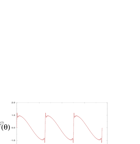
FIG. 2.: The first odd eigenfunction obtained from traditional stability analysis.

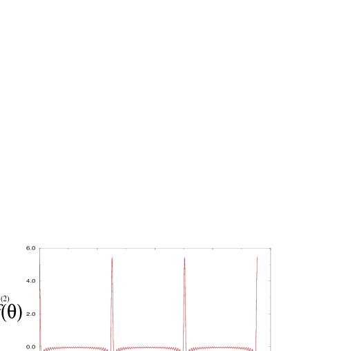
FIG. 3.: The first even eigenfunction obtained from traditional stability analysis.

FIG. 4.: The eigenvalues associated with perturbing the positions of the poles that consist the giant cusp. The largest eigenvalue is zero. The second, third, fourth and fifth eigenvalues are represented by a solid line, dot-dashed line, dotted line and dashed line respectively.

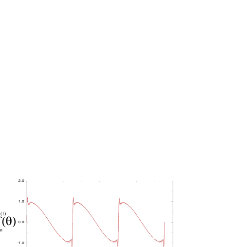
FIG. 5.: The first odd eigenfunction associated with perturbing the positions of the poles in the giant cusp.

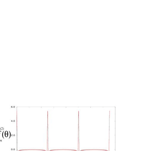
FIG. 6.: The first even eigenfunction associated with perturbing the positions of the poles in the giant cusp.

FIG. 7.: Spectrum of eigenvalues associated with the reaction of the poles in the giant cusp to the addition of new poles.

- [1] P. Pelce, Dynamics of Curved Fronts, (Academic press, Boston (1988))
- [2] A.-L. Barbási and H.E. Stanley, Fractal Concepts in Surface Growth (Cambridge University Press, 1995).
- [3] T. Viscek Fractal Growth Phenomena (World Scientific, Singapore, 1992).
- [4] O. Thual, U.Frisch and M. Henon, J. Physique, 46, 1485 (1985).
- [5] G.I. Sivashinsky, Acta Astronautica 4, 1177 (1977).
- [6] S. Gutman and G. I. Sivashinsky, Physica D43, 129 (1990).
- [7] O. Kupervasser, Z. Olami and I. Procaccia, Phys. Rev. Lett. 76, 146 (1996).
- [8] Z.Olami, B. Galanti, O. Kupervasser and I. Procaccia, Phys.Rev. E, 55, 2649 (1997).
- [9] Y. C. Lee and H. H Chen, Phys. Scr.,T 2,41 (1982).
- [10] G. Joulin, J. Phys. France, 50, 1069 (1989).
- [11] G. Joulin, Zh.Eksp. Teor. Fiz., 100, 428 (1990).
- [12] B. Galanti, O. Kupervasser, Z. Olami and I. Procaccia Phys. Rev. Lett. 80, 11 (1998).