Non-deterministic density classification with diffusive probabilistic cellular automata

Abstract

We present a probabilistic cellular automaton (CA) with two absorbing states which performs classification of binary strings in a non-deterministic sense. In a system evolving under this CA rule, empty sites become occupied with a probability proportional to the number of occupied sites in the neighborhood, while occupied sites become empty with a probability proportional to the number of empty sites in the neighborhood. The probability that all sites become eventually occupied is equal to the density of occupied sites in the initial string.

I Introduction

Cellular automata (CA) and other spatially-extended discrete dynamical systems are often used as models of complex systems with large number of locally interacting components. One of the primary problems encountered in constructing such models is the inverse problem: the question how to find a local CA rule which would exhibit the desired global behavior.

As a typical representative of the inverse problem, the so-called density classification task Gacs et al. (1987) has been extensively studied in recent years. The CA performing this task should converge to a fixed point of all 1’s if the initial configuration contains more 1’s than 0’s, and to a fixed point of all 0’s if the converse is true. While it has been proved Land and Belew (1995) that the two-state rule performing this task does not exist, solutions of modified tasks are possible if one allows more than one CA rule Fukś (1997), modifies specifications for the final configuration Capcarrère et al. (1996), or assumes different boundary condition Sipper et al. (1998). Approximate solutions have been studied in the context of genetic algorithms in one Mitchell et al. (1994) and two dimensions Morales et al. (2001).

In what follows, we will define a probabilistic CA which solves the density classification problem in the stochastic sense, meaning that the probability that all sites become eventually occupied is equal to the density of occupied sites in the initial string.

We will assume that the dynamics takes place on a one-dimensional lattice with periodic boundary conditions. Let $s_{i}(k)$ denotes the state of the lattice site $i$ at time $k$, where $i\in{\mathbf{Z}}$, $k\in{\mathbf{N}}$. All operations on spatial indices $i$ are assumed to be modulo $L$, where $L$ is the length of the lattice. We will further assume that $s_{i}(k)\in\{0,1\}$, and we will say that the site $i$ is occupied (empty) at time $k$ if $s_{i}(k)=1$ ($s_{i}(k)=0$).

The dynamics of the system can be described as follows: empty sites become occupied with a probability proportional to the number of occupied sites in the neighborhood, while occupied sites become empty with a probability proportional to the number of empty sites in the neighborhood, with all lattice sites updated simultaneously at each time step. To be more precise, let us denote by $P(s_{i}(k+1))|s_{i-1}(k),s_{i}(k),s_{i+1}(k))$ the probability that the site $s_{i}(k)$ with nearest neighbors $s_{i-1}(k),s_{i+1}(k)$ changes its state to $s_{i}(k+1)$ in a single time step. The following set of transition probabilities defines the aforementioned CA rule:

$$P(1|0,0,0) =0 \qquad P(1|0,0,1) =p$$

$$P(1|0,1,0) =1-2p \qquad P(1|0,1,1) =1-p$$

$$P(1|1,0,0) =p \qquad P(1|1,0,1) =2p$$

$$P(1|1,1,0) =1-p \qquad P(1|1,1,1) =1,$$ (1)

where $p\in(0,1/2]$ (the remaining eight transition probabilities can be obtained using $P(0|a,b,c)=1-P(1|a,b,c)$ for $a,b,c\in\{0,1\}$). The probabilistic CA defined by (I) can be defined explicitly if we introduce a set of iid random variables $\{X_{i}\}_{i=0}^{L}$ with probability distribution $P(X_{i}=1)=p$, $P(X_{i}=0)=1-p$, and another set $\{Y_{i}\}_{i=0}^{L}$ with probability distribution $P(Y_{i}=1)=2p$, $P(Y_{i}=0)=1-2p$. Dynamics of the rule (I) can then be described as

$$s_{i}(k+1)=X_{i}(1-s_{i-1})(1-s_{i})s_{i+1}$$

$$+(1-Y_{i})(1-s_{i-1})s_{i}(1-s_{i+1})$$

$$+(1-X_{i})(1-s_{i-1})s_{i}s_{i+1}$$

$$+X_{i}s_{i-1}(1-s_{i})(1-s_{i+1})$$

$$+Y_{i}s_{i-1}(1-s_{i})s_{i+1}$$

$$+(1-X_{i})s_{i-1}s_{i}(1-s_{i+1})$$

$$+s_{i-1}s_{i}s_{i+1}.$$ (2)

To make the above formula easier to read, we omitted the time argument, denoting $s_{i}(k)$ by $s_{i}$. After simplification and reordering of terms, we obtain

$$s_{i}(k+1)=s_{i}-s_{i}Y_{i}+X_{i}s_{i-1}+X_{i}s_{i+1}$$

$$+ (s_{i-1}s_{i}+s_{i}s_{i+1}-2s_{i-1}s_{i}s_{i+1}+s_{i-1}s_{i+1})(Y_{i}-2X_{i}).$$

II Difference and differential equations

The state of the system at the time $k$ is determined by the states of all lattice sites and is described by the Boolean random field $\mathbf{s}(k)=\{s_{i}(k):i=0\ldots L\}$. The Boolean field $\{\mathbf{s}(k):k=0,1,2,\ldots\}$ is then a Markov stochastic process. Denoting by $E_{\mathbf{s}(0)}$ the expectation of this Markov process when the initial configuration is $\mathbf{s}(0)$ we will now define the expected local density of occupied sites by $\rho_{i}(k)=E_{\mathbf{s}(0)}\left[s_{i}(k)\right]$. The expected global density will be defined as

$$\rho(k)=L^{-1}\sum_{i=0}^{L}\rho_{i}(k).$$ (4)

While both $\rho_{i}(k)$ and $\rho(k)$ depend on the initial configuration $\mathbf{s}(0)$, we will drop this dependence to simplify notation. We will assume that the initial configuration is exactly known (non-stochastic), hence $\rho(0)=\sum_{i=0}^{L}s_{i}(0)$ is the fraction of initially occupied sites.

Taking expectation value of both sides of (I), and taking into account that $E_{\mathbf{s}(0)}\left[Y_{i}-2X_{i}\right]=0$, we obtain the following difference equation

$$\rho_{i}(k+1)=\rho_{i}(k)+p\left(\rho_{i+1}(k)+\rho_{i-1}(k)-2\rho_{i}(k)\right).$$ (5)

After summing over all lattice sites this yields

$$\rho(k+1)=\rho(k),$$ (6)

which means that the expected global density should be constant, independently of the value of parameter $p$ and independently of the initial configuration $\mathbf{s}(0)$. We can therefore say that the probabilistic CA defined in (I) is analogous to conservative CA, i.e., deterministic CA which preserve the number of occupied sites Hattori and Takesue (1991); Boccara and Fukś (1998); Fukś (2000); Pivato (2001).

Note that up to now we have not made any approximations, i.e., both (5) and (6) are exact. We can, however, consider limiting behaviour of (5) when the physical distance between lattice sites and the size of the time step simultaneously go to zero, using a similar procedure as described in Lawniczak (2000). Let $x=\epsilon i$ and $t=\tau k$. Now in (5) we can replace $\rho(i,k)$ by $\rho(x,t)$, $\rho(i\pm 1,k)$ by $\rho(x\pm\epsilon,t)$ and $\rho(i,k+1)$ by $\rho(x,t+\tau)$, which results in the following equation:

$$\rho(r,t+\tau)=\rho(x,t)+p\left(\rho(x+\epsilon,t)+\rho(x-\epsilon,t)-2\rho(x,t)\right).$$

We will consider diffusive scaling in which time scales as a square of the spatial length, meaning that $\tau=\epsilon^{2}$. Taking Taylor expansion of the above equation in powers of $\epsilon$ up to the second order we obtain

$$\partial_{t}\rho=p\partial_{x}^{2}\rho,$$ (7)

i.e., the standard diffusion equation. Due to the form of (7), in what follows we will refer to the process defined in (I) as diffusive probabilistic cellular automaton (DPCA).

III Absorption probability

We will now present some simulation results illustrating dynamics of DPCA. Since main features of DPCA remain qualitatively the same for all values of the parameter $p$ in the interval $(0,1/2]$, we have chosen $p=0.25$ as a representative value to perform all subsequent simulations.

Let $N(k)=\sum_{i=1}^{L}s_{i}(k)$ be the number of occupied sites at time $k$. If we start with $N(0)=0$, then $N(k)=0$ for all $k>0$. Similarly, if $N(0)=L$, then $N(k)=L$ for all $k>0$. The DPCA has thus two absorbing states, corresponding to all empty sites (to be referred to as $\mathbf{0}$) and to all occupied sites (to be referred to as $\mathbf{1}$). If we start with $0<N(0)<L$, then the graph of $N(k)$ resembles a random walk, as shown in Figure 1.

Figure 1: Fraction of occupied sites $N(k)/L$ as a function of time $k$ for two sample trajectories starting from identical initial configuration with $N(0)=30$, $L=100$, $p=0.3$. The third, almost horizontal line represents average of $1000$ such trajectories.

Both sample trajectories shown there eventually end in the absorbing state, one of them in $\mathbf{0}$, another one in $\mathbf{1}$. This is a general property of the DPCA: regardless of the initial configuration, the system sooner or later ends up in one of the two absorbing states. Although the time required to reach the absorbing state can be large for a given realization of the process, the expected value of the number of time steps required to reach the absorbing state is finite, as it is the case for all finite absorbing Markov chains Kemeny and Snell (1960). Figure 2 illustrates this property for $L=100$ and the initial configuration with $30$ occupied sites clustered around the center, ie., located at $i=35,36,...,64$. All other sites are empty. We start with an assembly of $200$ of such initial configurations, all plotted as vertical lines in which black pixels represent occupied sites, while white pixels represent empty sites, as in Figure 2a. Each of these initial configurations evolves according to the DPCA rule, and after $k=100$ ($k=1000$) iterations they are again plotted as $200$ vertical lines in Figure 2b (2c). After $12000$ iterations all $200$ configurations reach absorbing states, as illustrated in Figure 2d. Obviously, some reach the state $\mathbf{1}$, while others $\mathbf{0}$, yet it turns out that the fraction of configurations which ended up in the state $\mathbf{1}$ is very close to $30\%$, the same as the fraction of occupied sites at $k=0$.

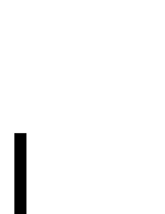
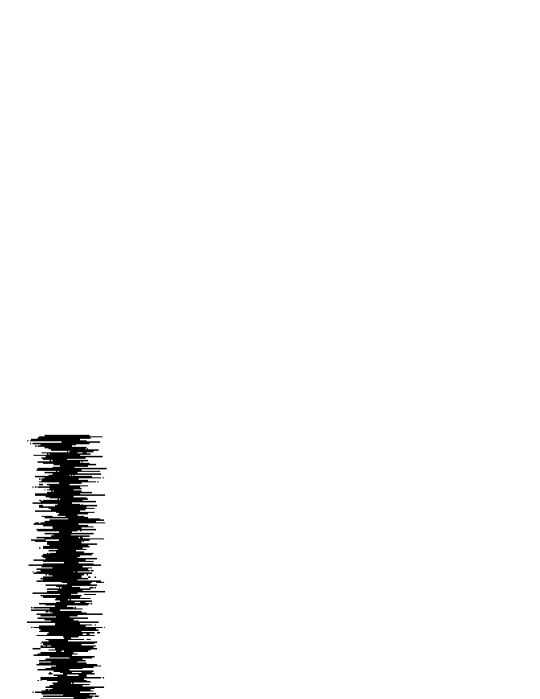
(a) (b)

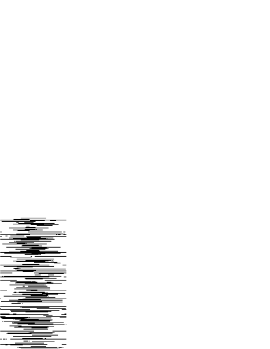
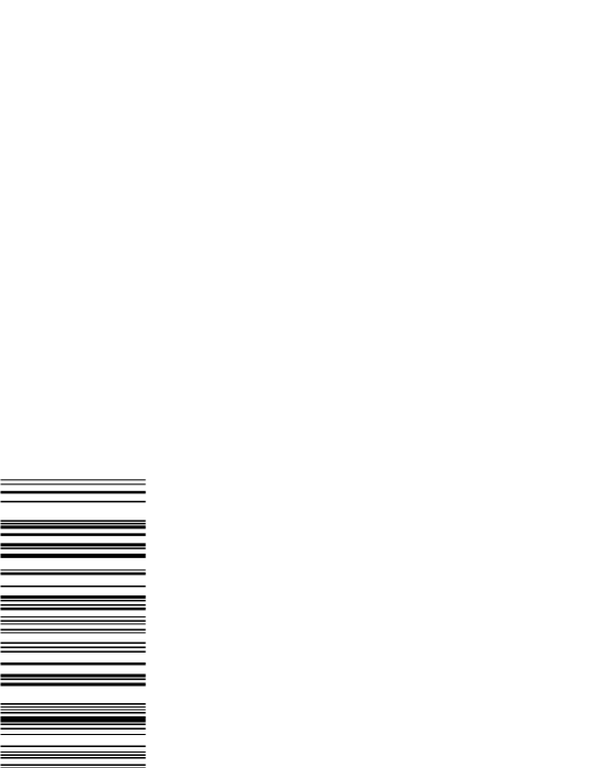
(c) (d)

Figure 2: Multiple realizations of the CA evolution at (a) $k=0$, (b) $k=100$, (c) $k=1000$ and (d) $k=12000$. Each vertical line corresponds to different realization of the process on $L=100$ lattice. Black pixels representing occupied sites and white pixels empty sites. 200 different realizations of the process are shown.

To explain this phenomenon, let us define $u_{N}(k)$ to be the probability that the number of occupied sites at time $k$ is $N$. Since the Markov process $\{\mathbf{s}(k):k=0,1,2,\ldots\}$ is finite and absorbing, no matter where the process starts, the probability that after $k$ steps it is in an absorbing state tends to $1$ as $k$ tends to infinity Kemeny and Snell (1960). This implies that

$$\lim_{k\rightarrow\infty}u_{N}(k)=0\mbox{\ if $N\neq 0$ and $N\neq L$},$$ (8)

$$\lim_{k\rightarrow\infty}\left(u_{L}(k)+u_{0}(k)\right)=1.$$ (9)

The expected global density, as defined in (4), is independent of $k$, hence

$$\rho(0)=L^{-1}E_{\mathbf{s}(0)}\left[N(k)\right]=L^{-1}\sum_{N=1}^{L}Nu_{N}(k).$$ (10)

Taking the limit $k\rightarrow\infty$ of both sides of the above equation, and using (8) and (9), we obtain

$$\lim_{k\rightarrow\infty}u_{L}(k)=\rho(0),$$ (11)

$$\lim_{k\rightarrow\infty}u_{0}(k)=1-\rho(0).$$ (12)

We have shown that the probability that the DPCA reaches the absorbing state $\mathbf{1}$ is equal to the initial fraction of occupied sites $\rho(0)$. The probability that it reaches $\mathbf{0}$ is $1-\rho(0)$. This is in agreement with the behavior observed in Figure 2.

The above can be viewed as a probabilistic generalization of the density classification process. In the standard (deterministic) version of the density classification problem we seek a CA rule which would converge to $\mathbf{1}$ ($\mathbf{0}$) if the fraction of occupied sites in the initial string is greater (less) than $1/2$, i.e.,

$$\lim_{k\rightarrow\infty}u_{L}(k)=\Theta(\rho(0)),$$ (13)

$$\lim_{k\rightarrow\infty}u_{0}(k)=\Theta(1-\rho(0)),$$ (14)

where $\Theta(\cdot)$ is the step function defined as $\Theta(x)=0$ if $x\leq 1/2$, and $\Theta(x)=1$ if $x>1/2$. Thus the difference between the deterministic and the probabilistic density classification introduced here is the replacement of the step function in (13-14) by the identity function in (11-12).

As opposed to deterministically determined outcome in the standard density classification process, in DPCA it is just more probable that the system reaches $\mathbf{1}$ then $\mathbf{0}$ if the fraction of occupied sites in the initial string is greater than $1/2$, and it is more probable that it reaches $\mathbf{0}$ then $\mathbf{1}$ if the converse is true. Additionally, DPCA can in some sense measure concentration of occupied sites in the initial string. If we want to know what is the initial density of occupied sites, we need to run DPCA many times with the same initial condition until it reaches the absorbing state, and observe how frequently it reaches $\mathbf{1}$. This frequency will approximate $N(0)/L$, with accuracy increasing with the number of experiments.

IV Time to absorption

Simulations shown in Figure 1 indicate that for large $k$ the system is typically in a state in which blocks of both empty and occupied sites are relatively long. We can use this observation to obtain the approximate dependence of the time required to reach the absorbing state on the density of initial configuration.

If we assume that in a given configuration all occupied sites are grouped in a few long continuous blocks, then the value of $N(k)$ cannot change too much in a single time step. For simplicity, let us assume that the only allowed values of $\Delta N(k)=N(k+1)-N(k)$ are $\{-2,-1,0,1,2\}$.

Figure 3: The average time required to reach the absorbing state $\langle T\rangle$ as a function of the initial density $\rho(0)=N(0)/L$ for $L=100$, $p=0.3$. Each data point ($+$) represents the average taken over $1000$ realizations of the process with identical initial configurations. The continuous line represents fitted parabola $\langle T\rangle=\alpha\rho(0)(1-\rho(0))$.

Since $\rho(k)$ is time-independent, the probability that $N(k)$ increases by a given amount should be equal to the probability that it decreases by the same amount in a single time step. In the agreement with the above, let us define $p_{j}$ as the probability that $\Delta N(k)$ takes the value $j$, so that $p_{j}$ is non-zero for $j\in\{-2,-1,0,1,2\}$, where $p_{-2}=p_{2}$, $p_{-1}=p_{1}$, and $2p_{2}+2p_{1}+p_{0}=1$. If $T_{z}$ denotes the expected time to reach the state $N(k)=0$ or $N(k)=L$ starting from $N(0)=z$, a simple argument Feller (1968) yields the difference equation which $T_{z}$ must satisfy

$$T_{z}=p_{2}T_{z+2}+p_{1}T_{z+1}+p_{0}T_{z}+p_{1}T_{z-1}+p_{2}T_{z-2}+1.$$ (15)

The solution of this equation satisfying boundary conditions $T_{0}=0$ and $T_{L}=0$ is given by

$$T_{z}=\alpha\,z(L-z)=\alpha\,L^{2}\rho(0)(1-\rho(0)),$$ (16)

where $\alpha=1/(8p_{2}+4p_{1})$, meaning that the mean time to absorption scales with lattice length as ${O}(L^{2})$. The above result would remain valid even if we allowed further jumps than $\pm 2$ (although the form of the coefficient $\alpha$ would be different).

In order to verify if this result holds for the DPCA, we performed a series of numerical experiments, computing the average time required to reach the absorbing state for 1000 realizations of the DPCA process, for a range of initial densities. Results are shown if Figure 3. One can clearly see that data points are aligned along a curve of parabolic shape, as expected from (16).

V Conclusion

The probabilistic CA introduced in this article solves the density classification problem in a non-deterministic sense. It is interesting to note that the DPCA conserves the average number of occupied sites, similarly as deterministic rules employed in solutions of related problems mentioned in the introduction. Indeed, conservation of the number of occupied sites is a necessary condition for density classification by CA if one allows modified output configuration, as recently shown in Capcarrère and Sipper (2001). This suggests that a wider class of probabilistic CA conserving $\rho(k)$ might be an useful paradigm in studying how locally interacting systems compute global properties, and certainly deserves further attention.

Acknowledgements

The author acknowledges financial support from the Natural Sciences and Engineering Research Council of Canada.

References

- Gacs et al. (1987) P. Gacs, G. L. Kurdymov, and L. A. Levin, Probl. Peredachi Inform. 14, 92 (1987).
- Land and Belew (1995) M. Land and R. K. Belew, Phys. Rev. Lett. 74, 5148 (1995).
- Fukś (1997) H. Fukś, Phys. Rev. E 55, 2081R (1997), eprint arXiv:comp-gas/9703001.
- Capcarrère et al. (1996) M. S. Capcarrère, M. Sipper, and M. Tomassini, Phys. Rev. Lett. 77, 4969 (1996).
- Sipper et al. (1998) M. Sipper, M. S. Capcarrère, and E. Ronald, Int. J. Mod. Phys. C 9, 899 (1998).
- Mitchell et al. (1994) M. Mitchell, J. P. Crutchfield, and P. T. Hraber, Physica D 75, 361 (1994).
- Morales et al. (2001) F. J. Morales, J. P. Crutchfield, and M. Mitchell, Parallel Comput. 27, 571 (2001).
- Hattori and Takesue (1991) T. Hattori and S. Takesue, Physica D 49, 295 (1991).
- Boccara and Fukś (1998) N. Boccara and H. Fukś, J. Phys. A: Math. Gen. 31, 6007 (1998), eprint arXiv:adap-org/9712003.
- Fukś (2000) H. Fukś, in Hydrodynamic Limits and Related Topics,, edited by S. Feng, A. T. Lawniczak, and R. S. Varadhan (AMS, Providence, RI, 2000), eprint arXiv:nlin.CG/0207047.
- Pivato (2001) M. Pivato (2001), preprint, eprint arXiv:math.DS/0111014.
- Lawniczak (2000) A. Lawniczak, Transport Theory and Statistical Physics 29, 261 (2000).
- Kemeny and Snell (1960) J. G. Kemeny and J. L. Snell, Finite Markov Chains (D. Van Nostrand Co., Princeton, NJ, 1960).
- Feller (1968) W. Feller, An Introduction to Probability Theory and Its Applications (Wiley and Sons, Inc., New York, 1968).
- Capcarrère and Sipper (2001) M. S. Capcarrère and M. Sipper, Phys. Rev. E 64, 036113 (2001).