Fluctuational transitions through a fractal basin boundary

Abstract

Fluctuational transitions between two co-existing chaotic attractors, separated by a fractal basin boundary, are studied in a discrete dynamical system. It is shown that the mechanism for such transitions is determined by a hierarchy of homoclinic points. The most probable escape path from the chaotic attractor to the fractal boundary is found using both statistical analyses of fluctuational trajectories and the Hamiltonian theory of fluctuations.

The mechanism of fluctuational escape from a chaotic attractor (CA) through a fractal basin boundary (FBB) represents one of the most challenging unsolved problems in fluctuation theory Kautz:87 ; Beale:89 ; Grassberger:89 ; Hamm:91 . The unpredictable and highly complex stochastic behavior of such systems arises in part from the presence of limit sets of complex geometrical structure, and in part from the fractality of the basin boundary Guken ; Ott . For this reason, the central question – whether or not there exists a generic mechanism for fluctuational transitions through the FBB – has remained unanswered. More specifically, it has remained unclear: (i) if boundary conditions can be found both on the CA and on the FBB; (ii) if there exits a unique escape path from the CA to the FBB; (iii) whether this path can be determined using the Hamiltonian theory of fluctuations; (iv) if there is any deterministic structure involved in the transition through the FBB itself; and (v) what effect is exerted by the noise intensity. If transitions across FBBs are characterised by general features, a knowledge of them could considerably simplify analyses of both stability and control for chaotic dynamical systems, which are problems of broad interdisciplinary interest Fradkov:98 ; Boccaletti:00 .

A promising approach to the solution of this problem is based on the analysis of fluctuations in the limit of very small noise intensity. In this limit, a stochastic dynamical system fluctuates to remote states along certain most probable deterministic paths Onsager:53 ; Dykman:92a ; Luchinsky:97 , corresponding to rays in the WKB-like asymptotic solution of the Fokker-Planck equation Freidlin:84 . The possibility of extending such an approach to chaotic systems, both continuous and discrete, was established earlier Kautz:87 ; Beale:89 ; Grassberger:89 ; Hamm:91 . It was shown also that the presence of homoclinic tangencies, causing the fractalization of the basins, causes a decrease in the activation energy Soskin:01 .

In this Letter we show that a generic mechanism of fluctuational transition between co-existing CAs separated by an FBB does exist, that it is determined by a hierarchy of homoclinic original saddles forming the homoclinic structure, and that there is a unique most probable escape path (MPEP) from the CA that approaches an accessible orbit on the fractal boundary.

To demonstrate the existence of this escape mechanism, we take as an example the two-dimensional map introduced by Holmes Holmes:79 . The properties of this map, including the structures both of its CA and of its locally disconnected FBB, are generic for a wide class of maps and flow systems Cartwright:51 ; Yorke:85a . It is this fact, taken with the results of our investigations of escape in other systems, that allows us to conclude that the escape mechanism described below is indeed a typical one. The Holmes map is

$$x_{n+1} = y_{n}$$ (1)

$$y_{n+1} = -b\,x_{n}+d\,y_{n}-y_{n}^{3}+\xi_{n},$$

where $\xi_{n}$ is zero-mean, white, Gaussian noise of variance $D$. Due to symmetry, the noise-free system (1) with $b=0.2$ and $2.0\leq d\leq 2.745$ has pairs of co-existing attractors, the basins of which are separated by a boundary that may be either smooth or fractal, depending on the choice of parameter values. We choose for our studies $b\,=\,0.2$ and $d\,=\,2.7$, which corresponds to there being two co-existing CAs separated by a locally disconnected FBB (see Fig. 1). The fractal dimension of the boundary has been determined numerically (dim = 1.84472) by using the “uncertainty exponent” technique introduced in Grebogi:85 . The chaotic attractors in (1) appear as the result of a period-doubling cascade and, for the parameters chosen, each of them consists of two disconnected parts.

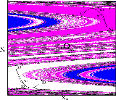
Figure 1: The co-existing chaotic attractors (filled black regions) and their basins of attraction represented by grey and white respectively. The accessible boundary saddle points of period 3 are shown by the small filled black circles labelled S3. Their stable manifolds are shown as full black lines. The saddle points of period 1 are shown by the crosses labelled S1. The saddle point at the origin is labelled O.

We have modelled the system (1) numerically, exciting it with weak noise, and have collected trajectories that include escape paths from one CA to the other, and also the corresponding realisations of noise that induced these transitions. By ensemble averaging a few hundred such escape trajectories and noise realisations, we have obtained the optimal escape path and the corresponding optimal force, which are shown in Fig. 2. The results of this statistical analysis allow us both to determine the boundary conditions near the CA and the FBB, and to demonstrate the uniqueness of the MPEP. It can be seen in particular that, in leaving the CA, the system (1) falls into a small neighbourhood of the saddle point of period 1 (S1) located between its two disconnected parts and having the multipliers $\rho_{1}=0.118975$ and $\rho_{2}=1.681025$. Its stable manifolds separate the parts of the CA, while the unstable ones belong to the CA. The system makes a few iterations in the neighbourhood of S1 (initial plateau in Fig. 2(a)) and then moves to the FBB in three steps, crossing it at a saddle point of period 3 (S3) with multipliers $\rho_{1}=0.001016$ and $\rho_{2}=7.875512$. Calculations have shown that, for the chosen parameter values, S3 lies within the FBB. Moreover, its stable manifold (solid black line in Fig. 1) is dense in the FBB and detaches the open neighborhood, including an attractor, from the FBB itself. This allows us to classify it as an accessible boundary point Grebogi:87 .

An analysis of the structure of escape paths inside the FBB has shown that the homoclinic saddle points play a key role in its formation. In the system (1), we observe an infinite sequence of saddle-node bifurcations of period $3,4,5,6,7...$, which occur at parameter values $d_{3}<d_{4}<d_{5}<d_{6}<d_{7}...\,$ and are caused by tangencies of the stable and unstable manifolds of the saddle point O at the origin. The homoclinic orbits appearing as a result of these bifurcations were classified earlier as original saddles, and it was also shown that their stable and unstable manifolds cross each other in a hierarchical sequence Grebogi:87 . To characterize this hierarchical relation between original saddles, it is reasonable to introduce a parameter $\mu$ equal to the ratio $\mid\,\ln(\rho_{1}(P))\,\mid/\ln(\rho_{2}(P))$, where $\rho_{1}$ and $\rho_{2}$ are the multipliers of a saddle point $P$. Calculations have shown that, for the original saddles of period $3,4,5,6,7,8...$ in (1), the following hierarchical sequence of index $\mu$ values occurs: $\mu_{3}=3.339,\,\mu_{4}=3.08,\,\mu_{5}=2.999,\,\mu_{6}=2.339,\,\mu_{7}=1.958,\,\mu_{8}=1.539$. Moreover, the values of index $\mu$ corresponding to the other homoclinic saddle cycles are close to zero. Correspondingly the probability of finding the system in their neighbourhood tends to zero.

These results allows us to infer features of a fluctuational transition through a locally disconnected FBB that are probably generic, as follows: (i) it always occurs through a unique accessible boundary point; and (ii) the original saddles forming the homoclinic structure of the system play a key role in the formation of the paths inside the FBB, the difference in their local stability defining the hierarchical relationship between them. Thus, we may claim that complicated structure of escape trajectories, caused by the thin homoclinic structure and their randomness, has in many respects a deterministic nature.

Having now understood the mechanism of escape, we can seek the MPEP. According to the Hamiltonian theory of fluctuations Kautz:87 ; Beale:89 ; Grassberger:89 ; Hamm:91 the MPEP is the path which minimizes the energy

$$S=\frac{1}{2}\sum_{n=1}^{N}\>{\xi^{T}_{n}\,\xi_{n}},$$ (2)

of the possible realizations of noise $\{\xi_{n}\}$ inducing a transition of the system (1) from the CA (with the initial condition on S1) to the FBB (with the final condition on the accessible orbit S3). The Lagrangian of the corresponding variational problem can be found following Grassberger:89 (cf. Dykman:90 ) in the form

$$L=\frac{1}{2}\sum_{n=1}^{N}\,{\bf{\xi^{T}_{n}}\,\xi_{n}}+\sum_{n=1}^{N}\,{\bf\lambda_{n}^{T}\,(x_{n+1}-f(x_{n})-\xi_{n})},$$

where (1) is taken into account using the Lagrange multiplier $\lambda_{n}$. Varying $L$ with respect to $\xi_{n}$, $\lambda_{n}$, and $x_{n}$, the following area-preserving map is obtained:

$$x_{n+1} = y_{n}$$

$$y_{n+1} = -b\,x_{n}+d\,y_{n}-y_{n}^{3}+\lambda_{n}^{y}$$ (3)

$$\lambda_{n+1}^{x} = (d-3x_{n+1}^{2})\,\lambda_{n}^{x}/b-\lambda_{n}^{y}/b$$

$$\lambda_{n+1}^{y} = \lambda_{n}^{x}$$

Equations (Fluctuational transitions through a fractal basin boundary) are supplemented by the following boundary conditions

$$\lim_{n\rightarrow-\infty}\lambda_{n}^{y}=0,\>\;(x_{n}^{0},y_{n}^{0})\in S1,\>\;(x_{n}^{1},y_{n}^{1})\in S3.$$ (4)

The MPEP is the minimum-energy heteroclinic trajectory connecting S1 to S3 in the phase space of (Fluctuational transitions through a fractal basin boundary). The solution of this boundary value problem is in general complicated, because of the presence of multiple local energy minima Luchinsky:02a induced by the complex geometrical structure of the unstable manifolds of S3 (see e.g. Graham:84a for a discussion). The solution of the boundary value problem involves a parameterization of the structure of the multiple local minima requiring, in turn, a proper parameterization of the unstable manifold in the vicinity of the initial conditions Beri:03 . The MPEP found by this method is shown in Fig. 2. It can be seen that, within the range shown by the vertical dotted lines in Fig. 2(a), the theoretical MPEP closely coincides with the path obtained by statistical analysis of escape trajectories in the Monte Carlo simulations. Note that no further action is required to bring the system to the other attractor once it has reached the accessible orbit of the FBB, i.e. once it has reached the points numbered 8 in Fig. 2(a) and (b); correspondingly, the optimal force measured in the numerical simulations (inset) falls back to zero.

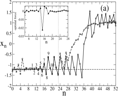
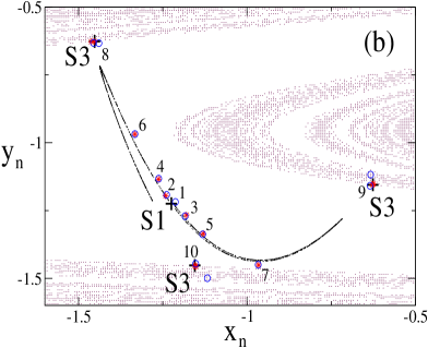
Figure 2: (a) the most probable escape path (dashed line) connecting the CA with the period-3 saddle cycle lying on the fractal boundary, obtained from the Monte-Carlo simulations with $D\,=\,10^{-5}.$ The optimal path found by the solution of the boundary-value problem is shown as a solid line. The $x$-coordinate of the saddle point S1 is shown by the horizontal dashed line. (b) A two-dimensional plot of the paths presented in (a) where the results obtained by solution of the the boundary value problem (consecutively numbered points indicated by circles, corresponding to the numbered points in (a)) coincide almost perfectly with those obtained by numerical simulation (stars). Inset in (a): the optimal force as determined in the numerical simulation.

The existence of an almost deterministic mechanism of transition across the FBB raises important questions about the effect of noise on this mechanism, and on the structure of escape trajectories inside the FBB. We have therefore used randomly chosen initial conditions in a very small neighborhood of the accessible point S3 through which escape occurs (see Fig. 2(b)). By definition, any arbitrarily small neighborhood of S3, lies within the FBB, and must contain points belonging to the basins of both attractors. Therefore the system can cross the FBB starting from a very small neighborhood of S3, even in the absence of noise. By collecting all such successful escape paths, we have calculated the probabilities for the system to pass via small neighborhoods of different original saddle cycles during its escape, both in the presence and absence of noise. As can be seen from Fig. 3, the corresponding probabilities demonstrate the same hierarchical interrelationship in both cases, which is determined by the value of index $\mu$ defined above. This structure is evidently robust with respect to noise-induced perturbations. The addition of noise causes a slight broadening of the distribution in Fig.  3 and a small increase of the probability for the system to escape via original saddles of larger period.

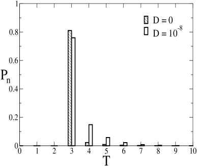
Figure 3: Probabilities of finding a fragment corresponding to the different period-$T$ original saddle cycle in the collected escape trajectories.

In conclusion, we have described the mechanism by which noise-induced escape occurs through a locally disconnected FBB. We have found the (unique) most probable escape path from a chaotic attractor to the fractal boundary, using both statistical analyses of fluctuational trajectories, and the Hamiltonian theory of fluctuations. We have shown that the original saddles forming the homoclinic structure play a key role in effecting the transition through the FBB itself. In particular, their local stability defines the hierarchical relationship between the probabilities for the system to pass via small neighborhoods of different original saddle cycles during its escape, both in the presence and in the absence of noise. We emphasize that the escape mechanism we have revealed must be applicable to the broad class of two dimensional maps and flows Holmes:79 ; Cartwright:51 ; Yorke:85a that exhibit the same type of FBB. For instance, one possible application of our results is to the development of an energy-optimal control scheme for the CO₂ laser, a discrete model of which demonstrates the type of FBB considered above Grigorieva .

The authors would like to thank Ulrike Feudel, Igor Khovanov and Suso Kraut for fruitful discussions. The work was supported by the Engineering and Physical Sciences Research Council (UK), the Russian Foundation for Fundamental Science, and INTAS.

References

- (1) R. L. Kautz, Phys. Lett. A 125, 315 (1987).
- (2) P. D. Beale, Phys. Rev. A 40, 3998 (1989).
- (3) P. Grassberger, J. Phys. A: Math. Gen. 22, 3283 (1989).
- (4) R. Graham, A. Hamm, and T. Tel, Phys. Rev. Lett. 66, 3089 (1991).
- (5) J. Guckenheimer and P. Holmes, Nonlinear Oscillations, Dynamical Systems, and Bifurcations of Vector Fields (New-York, Springer-Verlag, 1983).
- (6) E. Ott, Chaos in Dynamical Systems (Cambridge University Press, 2002).
- (7) A. L. Fradkov and A. Y. Pogromsky, Introduction to Control of Oscillations and Chaos, Series on Nonlinear Science A, Vol. 35 (Singapore, World Scientific, 1998).
- (8) S. Boccaletti, C. Grebogi, Y. C. Lai, H. Mancini and D. Maza, Phys. Rep 39, 103 (2000).
- (9) L. Onsager, and S. Machlup, Phys. Rev 91, 1505 (1953).
- (10) M. I. Dykman, P. V. E. McClintock, V. N. Smelyanskiy, N. D. Stein, and N. G. Stocks, Phys. Rev. Lett. 68, 2718 (1992).
- (11) D. G. Luchinsky, R. S. Maier, R. Mannella, P.V.E. McClintock, and D. L. Stein, Phys. Rev. Lett. 79, 3117 (1997); D. G. Luchinsky, J. Phys. A 30, L577 (1997); D. G. Luchinsky and P. V. E. McClintock, Nature 389, 463 (1997).
- (12) M. I. Freidlin and A. D. Wentzel, Random Perturbations in Dynamical Systems (Springer, New York, 1984).
- (13) S.M. Soskin, M. Arrayás, R. Mannella, and A.N. Silchenko, Phys. Rev. E. 63, 051111 (2001).
- (14) P. Holmes, Phil. Trans. R. Soc. (Lond.) A 292, 419 (1979).
- (15) M. L. Cartwright and J. E. Littlewood, Ann. Math. 54, 1 (1951); F. C. Moon and G. -X. Li, Phys. Rev. Lett. 55, 1439 (1985).
- (16) S.W. McDonald, C. Grebogi, E. Ott, and J.A. Yorke, Physica D 17, 125 (1985).
- (17) C. Grebogi, S. W. McDonald, E. Ott, and J. A. Yorke, Phys. Lett. A 99, 415 (1983).
- (18) C. Grebogi, E. Ott, and J.A. Yorke, Physica D 24, 243 (1987).
- (19) M. I. Dykman, Phys. Rev. A 42, 2020 (1990).
- (20) D. G. Luchinsky, S. Beri, R. Mannella, P.V.E. McClintock, and I.A. Khovanov, Int. J. Bifurcation and Chaos 12, 583 (2002).
- (21) R. Graham and T. Tel, Phys. Rev. Lett. 52, 9 (1984).
- (22) S. Beri, D. G. Luchinsky, R. Mannella, P. V. E. McClintock, submitted to Phys. Rev. E.
- (23) V. N. Chizhevsky, E. V. Grigorieva and S. A. Kashchenko, Opt. Commun. 133, 189 (1997).