Semiclassical theory of spin-orbit interaction in the extended phase space

Abstract

We consider the semiclassical theory in a joint phase space of spin and orbital degrees of freedom. The method is developed from the path integral using the spin-coherent-state representation, and yields the trace formula for the density of states. We discuss the limits of weak and strong spin-orbit coupling and relate the present theory to the earlier approaches.

1 Introduction

The subject of spin-orbit interaction in solid state physics has been attracting much attention recently due to potential applications in spin-based electronic devices [26, 12]. It has often proved advantageous, on the other hand, to exploit the semiclassical description of electrons in mesoscopic systems in the ballistic regime [28]. Hence there is a substantial interest in extending the semiclassical theory to include spin. Several attempts were made in the last decade in this direction. Littlejohn and Flynn [25] revised and improved the asymptotic theory of coupled wave equations and applied it to systems with standard spin-orbit coupling. Their approach, however, relies on a finite strength of the spin-orbit interaction, and thereby becomes invalid at the points in classical phase space where the interaction vanishes—the so-called mode-conversion points. Frisk and Guhr [13] found that in certain cases this problem can be corrected by a heuristic procedure. Bolte and Keppeler [5] studied the opposite situation when the interaction is weak. They derived the trace formula for the Dirac equation and Pauli equation with spin $1/2$. Based on the assumption that the orbital motion is not affected by spin, their approach was used to explain the anomalous magneto-oscillations in quasi-two-dimensional systems [20]. A comparative analysis of the above-mentioned semiclassical methods and their applications to specific systems can be found in [2].

In a new semiclassical approach to spin-orbit coupling [27] the orbital and spin degrees of freedom are combined in a joint (extended) phase space. Then the whole arsenal of the semiclassical methods developed for spinless systems can be applied there. The description of spin by continuous variables is achieved by using the basis of coherent states. After a path integral containing the spin and orbital coordinates is constructed, it can be evaluated in the stationary-phase approximation, yielding the semiclassical propagator or its trace.

A detailed investigation of the method of [27], with the focus on the trace formula for the density of states, is the subject of the present paper. We will argue that the earlier approaches can be put under one roof by this new theory. (A step in this direction was made in [36].) Our discussion will be limited to Hamiltonians linear in spin. For such systems, as we will show, the semiclassical treatment is valid not only in the large-spin limit, but also for a finite spin, including spin $1/2$.

We expect that the semiclassical method presented below can be effectively used in systems with relatively strong spin-orbit interaction, such as $p$-InAs or InGaAs-InAlAs heterostructures [18], or atomic nuclei [4]. Another field of application is molecular dynamics, where similar methods were developed to map the discrete electronic states to continuous variables and then to treat those semiclassically [33].

Our paper is organized as follows. In the introductory section 2 we briefly review the derivation of the trace formula without spin, starting from the path-integral representation for the propagator. Recently proposed by Sugita [32], this new procedure reproducing the well-known result of Gutzwiller [15] will later be generalized to include spin. In Sec. 3 we define the spin coherent states and write the quantum-mechanical partition function in the path-integral representation for a system with spin-orbit coupling. Sec. 4 is the main part of this work, where three versions of the trace formula are derived. In the first two instances we integrate over the spin variables in the path integral exactly and then apply the stationary-phase approximation. Consequently, for weak spin-orbit interaction (Sec. 4.1 and Appendix A) we obtain the generalization of the Bolte-Keppeler trace formula to arbitrary spin, and for strong coupling (Sec. 4.2) we recover, on a restricted basis, the result by Littlejohn and Flynn (at the moment we cannot recover their “no-name” phase). In the third case (Sec. 4.3) the path integral is evaluated by the stationary-phase method in both spin and orbital variables. Then, using Sugita’s approach, we express the oscillating part of the density of states as a sum over the periodic orbits in the extended phase space. Special attention is paid to the Solari-Kochetov phase correction [30, 22, 34] arising in the semiclassical limit of spin-coherent-state path integrals. In Sec. 4.4 we classify the regimes of weak, strong, and intermediate coupling, and show that the trace formula in the extended phase space works in all of them. (Appendix B illustrates explicitly the strong-coupling limit.) We also discuss and relax the large-spin applicability condition for the semiclassical approximation. As an application of the general theory, in Sec. 5 we study two systems with Rashba-type spin-orbit interaction [8] and the Jaynes-Cummings model [19].

2 Trace formula without spin

In this section we summarize some basic facts related to the semiclassical trace formula and present its derivation for systems without spin [32]. We consider a system described by the Schrödinger equation

$$\widehat{H}\,\psi_{k}=E_{k}\,\psi_{k}\,$$ (1)

with a discrete energy spectrum $\{E_{k}\}$. Its density of states $g(E)=\sum_{k}\delta(E-E_{k})$ can be subdivided into smooth and oscillating parts, i.e.,

$$g(E)=\widetilde{g}(E)+\delta g(E)\,.$$ (2)

From the semiclassical point of view, the smooth part $\widetilde{g}(E)$ is given by the contribution of all orbits with zero length and can be evaluated by the (extended) Thomas-Fermi theory [3]. Numerically it can be extracted by a Strutinsky averaging of the quantum spectrum [6].

In this paper we assume the smooth part to be known and will be interested in the oscillating part $\delta g(E)$, which is semiclassically approximated by the trace formula [15]

$$\delta g_{sc}(E)=\sum_{po}\mathcal{A}_{po}(E)\cos\left(\frac{1}{\hbar}\mathcal{S}_{po}(E)-\frac{\pi}{2}\sigma_{po}\right).$$ (3)

The sum here is over all classical periodic orbits ($po$), including all repetitions of each primitive periodic orbit ($ppo$). $\mathcal{S}_{po}(E)$ is the action integral and $\sigma_{po}$ is the Maslov index of a periodic orbit. The amplitude $\mathcal{A}_{po}(E)$ depends on the integrability and the continuous symmetries of the system. When all periodic orbits are isolated in phase space, the amplitude is given by [15]

$${\cal A}_{po}(E)=\frac{1}{\pi\hbar}\frac{T_{ppo}}{\sqrt{|\det(\widetilde{M}_{po}-I_{2(d-1)})|}},$$ (4)

where $T_{ppo}$ is the period of the primitive orbit, $\widetilde{M}_{po}$ is the stability matrix of the periodic orbit, and $d$ is the number of degrees of freedom. $I$ is the unit matrix, the subscript denotes the dimensionality of the space where $I$ acts. For two-dimensional systems $\sqrt{|\det(\widetilde{M}_{po}-I_{2})|}=2|\sin(\Lambda_{po}/2)|$, where $\Lambda_{po}$ is called the stability angle of a periodic orbit.

Recently Sugita [32] has proposed a re-derivation of Gutzwiller’s trace formula directly from the quantum partition function, avoiding the calculation of the semiclassical propagator. Since we utilize his approach in the following sections for systems with spin, we will briefly review it here. Sugita’s starting point is the quantum partition function (or the trace of the quantum propagator) in the path integral representation

$$Z(T)=\int\!\frac{{\cal D}[{\bf q}]{\cal D}[{\bf p}]}{(2\pi\hbar)^{d}}\,\exp\{i{\cal R}[{\bf q,p};T]/\hbar\}.$$ (5)

The path integral is calculated along closed paths $(\mathbf{q}(t),\mathbf{p}(t))$ in the $2d$-dimensional phase space over a time interval $T$:

$$\frac{{\cal D}[{\bf q}]{\cal D}[{\bf p}]}{(2\pi\hbar)^{d}}\equiv\lim_{N\to\infty}\prod_{l=1}^{N}\prod_{j=1}^{d}\left(\frac{dq_{j}(t_{l})dp_{j}(t_{l})}{2\pi\hbar}\right),\quad t_{l}=lT/N.$$ (6)

In (5)

$${\cal R}[{\bf q,p};T]\,=\oint_{0}^{T}\biggl{[}\frac{1}{2}({\bf p}\!\cdot\!{\bf\dot{q}}-{\bf q}\!\cdot\!{\bf\dot{p}})-\,{\cal H}({\bf q,p})\biggr{]}dt$$ (7)

is the Hamilton principal action function. ${\cal H}({\bf q,p})$ is the classical Hamiltonian, i.e., the Wigner-Weyl symbol of $\widehat{H}$. The action form ${\bf p}\cdot d{\bf q}$ can be antisymmetrized along the closed paths. The Fourier-Laplace transform of $Z(T)$ yields, after taking the imaginary part, the density of states

$$g(E)=-\frac{1}{\pi}\,\mathrm{Im}\left(\frac{1}{i\hbar}\int_{0}^{\infty}e^{iET/\hbar}\,Z(T)\,dT\,\right).$$ (8)

The path integral (5) receives its largest contributions from the neighborhoods of the classical paths, along which the principal function ${\cal R}$ is stationary according to Hamilton’s variational principle $\delta{\cal R}=0$. The first variation hereby yields the classical equations of motion

$$\dot{q}_{i}=\frac{\partial{\cal H}}{\partial p_{i}},\quad\dot{p}_{i}=-\frac{\partial{\cal H}}{\partial q_{i}}.$$ (9)

One may evaluate the integrations in (5) using the stationary-phase approximation, which becomes asymptotically exact in the classical limit ${\cal R}\gg\hbar$. The semiclassical approximation of the partition function $Z(T)$ then turns into a sum over all classical periodic orbits with fixed period $T$

$${\cal Z}_{sc}(T)=\sum_{po}e^{i{\cal R}_{po}/\hbar}\!\int\!\frac{{\cal D}[\mbox{{\boldmath$\eta$ \unboldmath}}\!\!]}{(2\pi)^{d}}\,\exp{\{i{\cal R}_{po}^{(2)}[\mbox{{\boldmath$\eta$ \unboldmath}}\!\!;T]\}}\,,$$ (10)

where ${\cal R}_{po}$ are the principal functions (7), evaluated now along the classical orbits. The functional of the second variations is

$${\cal R}_{po}^{(2)}[\mbox{{\boldmath$\eta$ \unboldmath}}\!\!,T]=\oint_{0}^{T}\left[\frac{1}{2}\mbox{{\boldmath$\eta$ \unboldmath}}\!\!\cdot{\cal J}\dot{\mbox{{\boldmath$\eta$ \unboldmath}}\!\!}-{\cal H}^{(2)}\right]\!dt$$ (11)

where $\eta$ is the $2d$-dimensional phase-space vector of small variations $\mbox{{\boldmath$\eta$ \unboldmath}}\!\!=(\mbox{{\boldmath$\lambda$ \unboldmath}}\!\!,\mbox{{\boldmath$\rho$ \unboldmath}}\!\!)=(\delta{\bf q},\delta{\bf p})/\sqrt{\hbar}$ and ${\cal J}=\left(\begin{array}[]{cc}0&I_{d}\!\\ \!\!-I_{d}&0\end{array}\right)$ is the $2d$-dimensional unit symplectic matrix. ${\cal H}^{(2)}$ is the second variation of the classical Hamiltonian ${\cal H}$, calculated along the periodic orbits:

$${\cal H}^{(2)}=\frac{1}{2}\sum_{i,j=1}^{d}\left[\lambda_{i}\lambda_{j}\frac{\partial^{2}{\cal H}}{\partial q_{i}\partial q_{j}}+2\lambda_{i}\rho_{j}\frac{\partial^{2}{\cal H}}{\partial q_{i}\partial p_{j}}+\rho_{i}\rho_{j}\frac{\partial^{2}{\cal H}}{\partial p_{i}\partial p_{j}}\right].$$ (12)

Note that ${\cal Z}_{sc}(T)$ does not include the contribution of the zero-length orbits.

After a stationary-phase evaluation of the Fourier-Laplace integral (8) with ${\cal Z}_{sc}(T)$ instead of $Z(T)$, one finally obtains Gutzwiller’s trace formula (3) where the actions ${\cal S}_{po}(E)={\cal R}_{po}$+$ET_{po}$ are calculated at fixed energy $E$ and the periods of the orbits are $T_{po}=dS_{po}/dE$. The monodromy matrix $M_{po}$ is defined by $\mbox{{\boldmath$\eta$ \unboldmath}}\!\!(T_{po})=M_{po}\,\mbox{{\boldmath$\eta$ \unboldmath}}\!\!(0)$ in terms of the solutions of the linearized equations of motion $\dot{\mbox{{\boldmath$\eta$ \unboldmath}}\!\!}={\cal J}\,\partial{\cal H}^{(2)}\!/\partial{\mbox{{\boldmath$\eta$ \unboldmath}}\!\!}$, which are purely classical. After removing the trivial parabolic block from $M_{po}$ that appears due to the time translation symmetry, one obtains the reduced $2(d-1)$-dimensional monodromy matrix $\widetilde{M}_{po}$. The latter enters formula (4) and since it contains information about the stability of periodic orbits [6] it is often referred to as the stability matrix. For the Maslov indices $\sigma_{po}$ Sugita has also given general formulae [32].

3 Spin coherent states and quantum partition function

We intend to generalize the path-integral representation for the partition function (5) to include the spin degree of freedom. The main issue then is to be able to describe spin on the quantum-mechanical level by a continuous variable. One can achieve this by using the overcomplete basis of spin coherent states. The path integral for a system with spin in the SU(2) spin-coherent-state representation originally appeared in a paper by Klauder [21] as an integral on the sphere $\mathbb{S}^{2}$. Kuratsuji et al. [23] have represented it as an integral over paths in the extended complex plane $\bar{\mathbb{C}}^{1}$.

The SU(2) coherent state $|z;s\rangle$ for spin $s$ is defined by

$$|z;s\rangle=(1+|z|^{2})^{-s}\exp(z\hat{s}_{+})\,|s,m_{s}=-s\rangle\,,$$ (13)

$$\hat{s}_{-}|s,m_{s}=-s\rangle=0\,,$$ (14)

where $z\in\bar{\mathbb{C}}^{1}$ is a complex number. The spin operators $\hat{s}_{\pm}=\hat{s}_{1}\pm i\hat{s}_{2}$ and $\hat{s}_{3}$ are the generators of the spin su(2) algebra:

$$[\hat{s}_{3},\hat{s}_{\pm}]=\pm\hat{s}_{\pm}\,,\qquad[\hat{s}_{+},\hat{s}_{-}]=2\hat{s}_{3}\,.\qquad$$ (15)

$|s,m_{s}\rangle$ are the eigenstates of $\hat{s}_{3}$. From the group-theoretical point of view, $s\in\mathbb{N}/2$ labels irreducible representations of SU(2).

The irreducibility, as well as the existence of the SU(2) invariant measure $d\mu_{s}$, ensures that the resolution of unity holds in the spin-coherent-state basis:

$$\int\!|z;s\rangle\langle z;s|\,d\mu_{s}(z^{*},z)=I_{2s+1}\,,$$

$$d\mu_{s}(z^{*},z)=\frac{2s+1}{\pi\,(1+|z|^{2})^{2}}d^{\,2}z\,.$$ (16)

This turns out to be the most important property of spin coherent states that allows for the path-integral construction. The measure $d\mu_{s}$ takes account of the curvature of the sphere $\mathbb{S}^{2}$. In what follows, we denote $|z;s\rangle$ simply by $|z\rangle$.

Let us now consider a quantum Hamiltonian with spin-orbit interaction

$$\widehat{H}=\widehat{H}_{0}+\widehat{H}_{s}=\widehat{H}_{0}(\hat{{\bf q}},\hat{{\bf p}})+\hbar\,\hat{{\bf s}}\cdot\widehat{{\bf C}}({\hat{\bf q}},\hat{{\bf p}})\,,$$ (17)

where $\hat{\bf s}=(\hat{s}_{1},\hat{s}_{2},\hat{s}_{3})$ and $\widehat{\bf C}=(\widehat{C}_{1},\widehat{C}_{2},\widehat{C}_{3})$ is a vector function of the coordinate and momentum operators $\hat{\bf q}$, $\hat{\bf p}$. Thereby we assume the most general form of spin-orbit interaction linear in spin. We write the expression for the respective quantum propagator in terms of a path integral in both the orbital variables ${\bf q,p}$ and the spin-coherent-state variables $z,z^{*}$. Imposing periodic boundary conditions on the propagation and thus integrating over closed paths, we arrive at the expression for the partition function [cf. (5)]:

$$Z(T)=\int\!\frac{{\cal D}[{\bf q}]{\cal D}[{\bf p}]}{(2\pi\hbar)^{d}}\>{\cal D}\mu_{s}[z^{*},z]\,\exp\,\{i{\cal R}[{\bf q,p},z^{*},z;T]/\hbar\}.$$ (18)

The Hamilton principal action function now includes the symplectic 1-form due to spin:

$${\cal R}[{\bf q,p},z^{*},z;T]=\oint_{0}^{T}\biggl{[}\frac{1}{2}({\bf p}\!\cdot\!{\bf\dot{q}}-{\bf q}\!\cdot\!{\bf\dot{p}})+\hbar s\,\frac{z\dot{z}^{*}-z^{*}\dot{z}}{i(1\!+\!|z|^{2})}-{\cal H}({\bf q,p},z^{*},z)\biggr{]}dt\,,$$ (19)

and the path integration in (18) is taken over the $2(d+1)$-dimensional extended phase space:

$$\frac{{\cal D}[{\bf q}]{\cal D}[{\bf p}]}{(2\pi\hbar)^{d}}\>{\cal D}\mu_{s}[z^{*},z]=\lim_{N\to\infty}\prod_{l=1}^{N}\prod_{j=1}^{d}\frac{dq_{j}(t_{l})dp_{j}(t_{l})}{2\pi\hbar}\,d\mu_{s}(z^{*}(t_{l}),z(t_{l}))\,,$$ (20)

where the time interval $T$ is divided into $N$ time steps $t_{l}=lT/N$.

The c-number Hamiltonian ${\cal H}({\bf q,p},z^{*},z)$ appearing in the integrand of (19) is

$${\cal H}({\bf q,p},z^{*},z)={\cal H}_{0}({\bf q,p})+{\cal H}_{s}({\bf q,p},z^{*},z)={\cal H}_{0}({\bf q,p})+\hbar s{\bf n}(z^{*},z)\cdot{\bf C}({\bf q},{\bf p})\,,$$ (21)

where ${\cal H}_{0}({\bf q,p})$ and ${\bf C}({\bf q,p})$ are the Wigner-Weyl symbols of the operators $\widehat{H}_{0}$ and $\widehat{{\bf C}}$, and ${\bf n}=(n_{1},n_{2},n_{3})=\langle z|\hat{\bf s}|z\rangle/s$ is the unit vector of dimensionless classical spin. Its components in terms of $z^{*}$ and $z$ are given by

$$n_{1}+in_{2}=2z^{*}/(1+|z|^{2}),\quad n_{3}=-(1-|z|^{2})/(1+|z|^{2}).$$ (22)

One may recognize the stereographic projection from a point ${\bf n}$ on the unit Bloch sphere onto a point $(\mathrm{Re}\>z,-\mathrm{Im}\>z)$ on the complex plane, whereby the south pole is mapped onto its origin $z=0$.

We remark that the choice of the c-number Hamiltonian is not unique and, in the discretized path integral, is linked to a specific discretization prescription [24]. For symbolic manipulations in the continuous limit, it is often convenient to use the Wigner-Weyl symbol of the quantum Hamiltonian as the c-number Hamiltonian. Note, however, that $s{\bf n}$ is the covariant symbol of the spin operator $\hat{\mathbf{s}}$, and not the Wigner-Weyl symbol. The consequences of the present choice of ${\cal H}({\bf q,p},z^{*},z)$ (21) for the semiclassical theory are discussed in Sec. 4.4.

4 Semiclassics with spin-orbit coupling

In this section we consider the semiclassical approach for systems with spin-orbit interaction. We begin with the limit of weak coupling (Sec. 4.1), calculating the spin part of the path integral exactly. The trace formula we obtain is a generalization of the results by Bolte and Keppeler [5] to arbitrary spin. A similar approach leads, under certain restrictions, to the trace formula in the adiabatic (strong-coupling) limit (Sec. 4.2), that was studied by Littlejohn and Flynn [25]. In Sec. 4.3 we present a new method that treats both orbital and spin degrees of freedom semiclassically [27]. With the latter approach one can go beyond the limits of weak and strong coupling. The relationship between the methods, in connection with the coupling strength, is analyzed in Sec. 4.4.

4.1 Weak-coupling limit: quantum-mechanical treatment of spin

We derive here the semiclassical trace formula for the Hamiltonian (17) in the asymptotic limit $\hbar\rightarrow 0$. In addition to the standard semiclassical requirement ${\cal R}/\hbar\gg 1$, which is automatically fulfilled, this limit also implies that the spin-orbit interaction energy is small:

$$|{\cal H}_{s}({\bf q,p},z^{*},z)|\ll|{\cal H}_{0}({\bf q,p})|,$$ (23)

i.e., the system is in the weak-coupling regime.

It is convenient to separate the terms that explicitly contain $\hbar$ in the Hamilton principal action function (19). Representing

$${\cal R}[{\bf q},{\bf p},z^{*},z;T]={\cal R}_{0}[{\bf q},{\bf p};T]+\hbar s{\cal R}_{1}[{\bf q},{\bf p},z^{*},z;T],$$ (24)

where the unperturbed part ${\cal R}_{0}$ is given by (7) with the Hamiltonian ${\cal H}_{0}({\bf q,p})$ and

$${\cal R}_{1}[{\bf q},{\bf p},z^{*},z;T]=\oint_{0}^{T}\biggl{[}\frac{z\dot{z}^{*}-z^{*}\dot{z}}{i(1\!+\!|z|^{2})}-{\bf n}(z^{*},z)\cdot{\bf C}({\bf q},{\bf p})\biggr{]}dt\,,$$ (25)

we can write the partition function (18) in the form

$$Z(T)=\int\frac{{\cal D}[{\bf q}]{\cal D}[{\bf p}]}{(2\pi\hbar)^{d}}{\cal M}_{s}[{\bf q},{\bf p};T]\exp\left\{i{\cal R}_{0}[{\bf q},{\bf p};T]/\hbar\right\}$$ (26)

with

$${\cal M}_{s}[{\bf q},{\bf p};T]=\int{\cal D}\mu_{s}[z^{*},z]\exp\left\{is{\cal R}_{1}[{\bf q},{\bf p},z^{*},z;T]\right\}.$$ (27)

Now we can evaluate $Z(T)$ in the stationary-phase approximation in ${\bf q}$ and ${\bf p}$. Since $s{\cal R}_{1}\ll{\cal R}_{0}/\hbar$ in the case under consideration, ${\cal M}_{s}[{\bf q},{\bf p};T]$ is a slowly varying functional of ${\bf q}$ and ${\bf p}$ and need not be taken into account when evaluating the stationary-phase condition. Applying the results of Sec. 2, we obtain the semiclassical approximation to the partition function as a sum over the unperturbed periodic orbits (determined entirely by ${\cal H}_{0}$)

$$Z_{sc}(T)=\sum_{po}{\cal M}_{po}(T)\,{\cal A}^{(0)}_{po}(T)\exp\left\{i{\cal R}^{(0)}_{po}/\hbar-\nu^{(0)}_{po}\pi/2\right\},$$ (28)

where ${\cal A}^{(0)}_{po}$, $\;\nu^{(0)}_{po}$, ${\cal R}^{(0)}_{po}\equiv{\cal R}_{0}[{\bf q}^{(0)}_{po},{\bf p}^{(0)}_{po};T]$, and the modulation factor ${\cal M}_{po}(T)\equiv{\cal M}_{s}[{\bf q}^{(0)}_{po},{\bf p}^{(0)}_{po};T]$ are evaluated for the unperturbed trajectory. Performing the Fourier-Laplace transform (8) (also in stationary-phase approximation) we arrive at the trace formula in the weak-coupling limit (WCL)

$$\delta g_{sc}^{\mathrm{WCL}}=\sum_{po}{\cal M}_{po}(E)\,{\cal A}^{(0)}_{po}(E)\cos\left\{i{\cal S}^{(0)}_{po}/\hbar-\sigma^{(0)}_{po}\pi/2\right\},$$ (29)

which differs from the unperturbed trace formula for ${\cal H}_{0}$ only by the presence of the modulation factor ${\cal M}_{po}(E)\equiv{\cal M}_{po}(T^{(0)}(E))$ with $T^{(0)}(E)=d{\cal S}_{po}^{(0)}/dE$.

The modulation factor is determined in Appendix A by a direct evaluation of the path integral (27). For a Hamiltonian linear in spin, the problem is effectively reduced to the calculation of the spin partition function in the time-dependent external magnetic field ${\bf C}({\bf q(t)},{\bf p(t)})\equiv(2\,{\rm Re}f(t),-2\,{\rm Im}f(t),2A(t))$, determined by the path $({\bf q(t)},{\bf p(t)})$. Then for a periodic orbit one finds

$${\cal M}_{po}(E)=\frac{\sin[(s+1/2)\,\eta(E)]}{\sin[\eta(E)/2]}$$ (30)

with

$$\eta(E)=\int_{0}^{T^{(0)}}dt\,\{2A^{(0)}(t)-[(f^{(0)}(t))^{*}z+f^{(0)}(t)z^{*}]\}.$$ (31)

$z^{*}(t)$ and $z(t)$ are to be found from the first-order differential equation

$$\dot{z}=-i[2A^{(0)}(t)z+f^{(0)}(t)-(f^{(0)}(t))^{*}z^{2}],\quad z(0)=z(T),$$ (32)

which is simply the precession equation $\dot{{\bf n}}={\bf C}^{(0)}\times{\bf n}$, ${\bf n}(0)={\bf n}(T)$ for the classical spin vector ${\bf n}$ [Eq. (22)]. This equation is angle-preserving, i.e., it rotates the Bloch sphere without deforming it. Thus, the orientations of the Bloch sphere at $t=0$ and $t=T$ are related by a rotation about some axis. The angle of rotation is $\eta(E)$ (Appendix A). The choice of initial condition ${\bf n}(0)$ along this axis corresponds to a periodic solution (cf. [36]). Thus, (32) has two periodic solutions, whose $\eta(E)$ have opposite signs. Nevertheless, ${\cal M}_{po}(E)$ is well defined. Note that $\eta(E)$ is equal to the part ${\cal R}_{1}[{\bf q}^{(0)}_{po},{\bf p}^{(0)}_{po},z^{*},z;T^{(0)}]$ of the Hamilton principal action function calculated along the periodic $z^{*}(t)$ and $z(t)$. Although we are able to give a classical interpretation to the ingredients of ${\cal M}_{po}(E)$, no stationary-phase approximation was used in its derivation.

In the absence of spin-orbit interaction or external magnetic fied one finds ${\cal M}_{po}(E)\!=2s+1$, i.e., the unperturbed trace formula is multiplied by the spin degeneracy factor.

For $s=1/2$ the modulation factor ${\cal M}_{po}(E)$ was derived in [5] by a different method, which, as ours, treats the spin degrees of freedom on the quantum-mechanical level.

Clearly, when the weak-coupling condition (23) breaks down, the trace formula (29) is no longer valid. Indeed, in this case ${\cal R}_{1}$ is large, and ${\cal M}_{s}[{\bf q},{\bf p};T]$ will influence the stationary-phase condition for the integral (26).

Note that the representation of terms in the WCL trace formula as a product of the unperturbed part and the modulation factor [Eq. (29)] remains valid even when the Hamiltonian is nonlinear in spin. However, the simple expression for the modulation factor Eq. (30) is specific to the Hamiltonian linear in spin.

4.2 Adiabatic limit: strong coupling

With an exact integration over the spin degrees of freedom in the path integral we can also derive the trace formula in the adiabatic limit. This limit is defined by the requirement

$$|{\bf C(q,p)}|\gg T^{-1}_{\mathrm{orb}},$$ (33)

where $T_{\mathrm{orb}}$ is the period of the orbital motion. Since $|{\bf C}|$ is the frequency of precession of the classical spin about the instantaneous magnetic field ${\bf C}$, Eq. (33) means that the spin motion is much faster than the orbital motion. The results of this section will be most useful in the strong-coupling limit (SCL) $|{\cal H}_{s}|\sim|{\cal H}_{0}|$ or $|{\bf C}|\sim|{\cal H}_{0}|/\hbar$, where (33) is automatically satisfied. Formally speaking, the SCL can be stated as the double-limit $\hbar\to 0$, $|{\bf C}|\to\infty$ with $\hbar|{\bf C}|=\mathrm{const}$ (cf. [5]).

We start with the representation (26) for the partition function and write the prefactor in the form (Appendix A)

$${\cal M}_{s}[{\bf q},{\bf p};T]=\frac{\sin\{(s+1/2)\,\eta\,[\mathbf{q,p};T]\}}{\sin\{\eta\,[\mathbf{q,p};T]/2\}}=\sum_{m_{s}=-s}^{s}\exp\{im_{s}\eta\,[\mathbf{q,p};T]\}.$$ (34)

Then $Z(T)$ becomes a sum over polarizations

$$Z(T)=\sum_{m_{s}=-s}^{s}\int\frac{{\cal D}[{\bf q}]{\cal D}[{\bf p}]}{(2\pi\hbar)^{d}}\exp\left\{i{\cal R}_{0}[\mathbf{q,p};T]/\hbar+im_{s}\eta\,[\mathbf{q,p};T]\right\},$$ (35)

where the path integrals will be calculated by the stationary phase. The functional $\eta\,[\mathbf{q,p};T]$ is given by [cf. (31)]

$$\eta\,[\mathbf{q,p};T]=\int_{0}^{T}dt\,\{2A-[f^{*}z+fz^{*}]\}$$ (36)

with $f=|{\bf C}|\sin\theta_{C}e^{-i\phi_{C}}$ and $A=(|{\bf C}|/2)\cos\theta_{C}$ in terms of the polar angles $\theta_{C}$, $\phi_{C}$ of the vector ${\bf C}$. The trajectory $z(t)$ is one of the two periodic solutions of the equation

$$\dot{{\bf n}}={\bf C}\times{\bf n},\quad|{\bf n}|=1,$$ (37)

which can be solved approximately in the adiabatic limit. We look for the solution in the form ${\bf n}={\bf n}^{(0)}+{\bf n}^{(1)}$, where ${\bf n}^{(0)}\parallel{\bf C}$ and ${\bf n}^{(1)}\perp{\bf C}$. Assuming ${\bf n}^{(1)}\sim{\bf n}^{(0)}/(|{\bf C}|\,T_{\mathrm{orb}})\ll{\bf n}^{(0)}$, we obtain

$${\bf n}^{(0)}=\pm\frac{{\bf C}}{|{\bf C}|},\quad{\bf n}^{(1)}=\mp\frac{{\bf n}^{(0)}\times\dot{{\bf n}}^{(0)}}{|{\bf C}|}.$$ (38)

Then (36) gives us the phase

$$m_{s}\,\eta\,[\mathbf{q,p};T]=-m_{s}\,\int_{0}^{T}|{\bf C}|\,dt\,+\,\varphi_{B}^{(m_{s})}\,+\,\mathcal{O}(|{\bf C}|\,T_{\mathrm{orb}})^{-1}.$$ (39)

Here the second term is the Berry phase

$$\varphi_{B}^{(m_{s})}=m_{s}\int_{0}^{T}(1+\cos\theta_{C})\,\dot{\phi}_{C}\,dt.$$ (40)

When the path integrals (35) for $Z(T)$ are evaluated by stationary phase, the Berry phase $\varphi_{B}^{(m_{s})}\sim 1$ does not play a role in the determination of the stationary-phase point. In the SCL, i.e., when $|{\bf C}|\sim|{\cal H}_{0}|/\hbar$, the first term of (39) must be varied together with ${\cal R}_{0}/\hbar$ in order to derive the stationary-phase condition. Then after the standard procedure (Sec. 2) we obtain the trace formula

$$\delta g_{sc}^{\mathrm{SCL}}=\sum_{m_{s}=-s}^{s}\delta g_{sc}^{(m_{s})},$$ (41)

where each polarized density of states $\delta g_{sc}^{(m_{s})}$ is given by (3) with the classical dynamics controlled by the effective Hamiltonian

$${\cal H}_{\mathrm{eff}}^{(m_{s})}\mathbf{(q,p)}={\cal H}_{0}\mathbf{(q,p)}+m_{s}\hbar|\mathbf{C(q,p)}|$$ (42)

and the Berry phase added. An independent semiclassical derivation of this result is given in Appendix B.

Actually, this result is valid only if ${\bf C(q,p)}$ depends on either $q_{j}$ or $p_{j}$, but not both, for each $j=1,\ldots,d$. In the latter case such symbolic manipulations with path integrals do not seem to be valid, and, as a result, the “no-name” term found by Littlejohn and Flynn [25] is missing. The problem of recovering this term in the path-integral approach has been known for some time and was already mentioned in Ref. [25]. Making some heuristic assumptions, Fukui [14] reproduced the no-name term for the Jaynes-Cummings model in a framework similar to ours. It is not clear to us at this stage, whether his approach can be generalized to a wider class of Hamiltonians. We suppose that this term emerges due to the operator ordering, and hope to recover it making a careful analysis of the continuous limit of the path integral.

It may happen that the adiabatic condition (33) is fulfilled in the WCL. The trace formula is well defined if the limit $\hbar|{\bf C}|/{\cal H}_{0}\rightarrow 0$ is taken before the limit $|{\bf C}|\,T_{\mathrm{orb}}\rightarrow\infty$. Hence, $m_{s}\,\eta\,[\mathbf{q,p};T]$ does not contribute to the determination of the stationary point, and the orbital motion is governed entirely by ${\cal H}_{0}$. The results of the previous section will be recovered with $\eta(E)$ given by (39), i.e., the fast spin precession can be removed from $\eta(E)$ in the adiabatic limit.

We note that expression (39) becomes invalid if the adiabatic condition (33) breaks down anywhere along the periodic orbit. In particular, this occurs in the mode-conversion points defined by $\mathbf{C(q,p)}=0$.

4.3 Semiclassics in the extended phase space

In the present approach, proposed recently in [27], both the orbital and spin degrees of freedom are treated semiclassically. For the formal derivation we assume the standard semiclassical requirements of large action ${\cal R},{\cal S}\gg\hbar$ and large spin angular momentum, i.e.,

$$S\equiv\hbar s\gg\hbar.$$ (43)

Later the second condition will be dropped. The spin-orbit coupling is allowed to be arbitrary now. Moreover, we show in Sec. 4.4 that the WCL trace formula (29) and the SCL trace formula (41) can be reproduced within the approach of [27].

In Sec. 2 we presented the derivation of the spinless trace formula starting from the quantum partition function. Here we apply the same scheme to the spin-dependent $Z(T)$ of (18) with the c-number Hamiltonian (21) responsible for the classical dynamics. At the end we should obtain the trace formula in its standard form (3). However, all its elements (periodic orbits, their actions, periods, and stabilities) are to be found from the dynamics in the extended phase space ${\bf q},{\bf p},z^{*},z$. In what follows we show how these ingredients can be determined.

The first step is to obtain the classical equations of motion from the variational principle $\delta{\cal R}[{\bf q},{\bf p},z^{*},z]=0$, where, in particular, $z^{*}$ and $z$ are varied independently. These generalized Hamilton equations are

$$\dot{q}_{i}=\frac{\partial{\cal H}}{\partial p_{i}},\quad\dot{p}_{i}=-\frac{\partial{\cal H}}{\partial q_{i}},$$ (44)

$$\dot{z}^{*}=i\frac{(1+|z|^{2})^{2}}{2S}\frac{\partial{\cal H}}{\partial z},\quad\dot{z}=-i\frac{(1+|z|^{2})^{2}}{2S}\frac{\partial{\cal H}}{\partial z^{*}}.$$ (45)

We emphasize that these equations describe the coupled dynamics of spin and orbital degrees of freedom and collectively determine the periodic orbits in the extended phase space.

The second pair of equations are not redundant, as may appear. Actually, they prove the expected property that $z^{*}$ is indeed the complex conjugate of $z$ along the classical paths. After we have established this, we can rewrite Eqs. (45) in terms of the real variables $v=\mathrm{Im}\,z^{*}=-\mathrm{Im}\,z$ and $u=\mathrm{Re}\,z^{*}=\mathrm{Re}\,z$ as

$$\dot{v}=\frac{(1\!+\!|z|^{2})^{2}}{4S}\frac{\partial{\cal H}}{\partial u},\quad\dot{u}=-\frac{(1\!+\!|z|^{2})^{2}}{4S}\frac{\partial{\cal H}}{\partial v}.$$ (46)

These two equations are equivalent to

$$\dot{{\bf n}}={\bf C}\times{\bf n},$$ (47)

with ${\bf n}$ given by (22). (As was already mentioned, the WCL equation (32) is of the same form as (45), if ${\cal H}$ is calculated along the unperturbed orbits.) It is worth noting that the equations of motion (44), (46) can be formulated in terms of the generalized Poisson bracket

$$\dot{{\cal F}}=\left\{{\cal F},{\cal H}\right\}=\frac{\partial{\cal F}}{\partial{\bf q}}\frac{\partial{\cal H}}{\partial{\bf p}}-\frac{\partial{\cal F}}{\partial{\bf p}}\frac{\partial{\cal H}}{\partial{\bf q}}+\frac{(1+u^{2}+v^{2})^{2}}{4S}\left(\frac{\partial{\cal F}}{\partial v}\frac{\partial{\cal H}}{\partial u}-\frac{\partial{\cal F}}{\partial u}\frac{\partial{\cal H}}{\partial v}\right)$$ (48)

for any function ${\cal F}$ of the extended-phase-space coordinates.

According to (19), the action along a periodic orbit is

$${\cal S}_{po}(E)=\oint_{0}^{T(E)}\biggl{[}\frac{1}{2}({\bf p}\!\cdot\!{\bf\dot{q}}-{\bf q}\!\cdot\!{\bf\dot{p}})+2S\,\frac{u\dot{v}-v\dot{u}}{1\!+\!u^{2}+\!v^{2}}\biggr{]}dt.$$ (49)

The functional of the second variations ${\cal R}_{po}^{(2)}[\mbox{{\boldmath$\eta$ \unboldmath}}\!\!,T]$ is still given by (11) with

$$\mbox{{\boldmath$\eta$ \unboldmath}}\!\!=(\mbox{{\boldmath$\lambda$ \unboldmath}}\!\!,\nu,\mbox{{\boldmath$\rho$ \unboldmath}}\!\!,\xi)=\frac{1}{\sqrt{\hbar}}\left(\delta{\bf q},\,\frac{2\sqrt{S}\,\delta v}{1+u^{2}+v^{2}},\,\delta{\bf p},\,\frac{2\sqrt{S}\,\delta u}{1+u^{2}+v^{2}}\right)\!,$$ (50)

as well as the $2(d+1)$-dimensional unit symplectic matrix ${\cal J}$ and the second variation of the classical Hamiltonian (21)

$${\cal H}^{(2)} = \frac{1}{2}\sum_{i,j}\left[\lambda_{i}\lambda_{j}\frac{\partial^{2}{\cal H}}{\partial q_{i}\partial q_{j}}+2\lambda_{i}\rho_{j}\frac{\partial^{2}{\cal H}}{\partial q_{i}\partial p_{j}}+\rho_{i}\rho_{j}\frac{\partial^{2}{\cal H}}{\partial p_{i}\partial p_{j}}\right]$$ (51)

$$+\,\frac{1}{2}(\nu^{2}+\xi^{2})\,\left(-u\,C_{1}-v\,C_{2}+C_{3}\right)$$

$$+\,\sqrt{S}\,\frac{(1+|z|^{2})}{2}\left(\nu\frac{\partial{\bf n}}{\partial v}+\xi\frac{\partial{\bf n}}{\partial u}\right)\cdot\sum_{j}\left(\lambda_{j}\frac{\partial{\bf C}}{\partial q_{j}}+\rho_{j}\frac{\partial{\bf C}}{\partial p_{j}}\right)\!.$$

The stability matrices and the Maslov indices are determined by the linearized dynamics $\dot{\mbox{{\boldmath$\eta$ \unboldmath}}\!\!}={\cal J}\,\partial{\cal H}^{(2)}\!/\partial{\mbox{{\boldmath$\eta$ \unboldmath}}\!\!}$, as usual [32].

There is, however, one component of the trace formula which is absent for spinless systems. It is the quantum phase correction that emerges in the semiclassical limit of the spin-coherent-state path integral [31]. Originally derived by Solari [30], Kochetov [22], and Vieira and Sacramento [34] for the semiclassical spin propagator, it is given by

$$\varphi^{SK}(T)=\frac{1}{2}\int_{0}^{T}B(t)dt,$$ (52)

where

$$B(t)=\frac{1}{2}\left[\frac{\partial}{\partial z^{*}}\frac{\left(1+|z|^{2}\right)^{2}}{2S}\frac{\partial{\cal H}}{\partial z}+\mathrm{c.c.}\right]$$ (53)

is evaluated along the classical path. Being purely of a kinematic nature, this phase plays the role of a normalization [22]. For the Hamiltonian (21) we find

$$B(t)=-uC_{1}-vC_{2}+C_{3}=2A(t)-[(f(t))^{*}z+f(t)z^{*}].$$ (54)

In the semiclassical limit of the partition function (18) the Solari-Kochetov phase is calculated along the periodic orbits. Since $\varphi^{SK}\sim\hbar^{0}$, this phase survives the Fourier-Laplace transform from $T$ to $E$ without affecting the stationary-phase condition and thus enters the trace formula:

$$\delta g_{sc}(E)=\sum_{po}\mathcal{A}_{po}(E)\cos\left(\frac{1}{\hbar}\mathcal{S}_{po}(E)+\varphi^{SK}_{po}(E)-\frac{\pi}{2}\sigma_{po}\right).$$ (55)

Note that, as follows from (54), $(1/2)\,\eta(E)$ in the WCL result (30) corresponds to the semiclassical Solari-Kochetov phase.

4.4 Applicability conditions and coupling regimes

We now will show that the semiclassical approach of the previous section is not restricted to large spin, provided that the Hamiltonian is linear in spin. Thus, we will go beyond the formal limit (43) and present the arguments justifying this step. We also identify the possible regimes of weak, strong, and intermediate coupling that are unified within the semiclassical treatment of the extended phase space.

The trace formula (55) results from a stationary-phase evaluation of the path integral (18) for the partition function. In the discretized version one finds the stationary-phase points in the space of $(2d+2)N$ variables $\mathbf{q}(t_{l})$, $\mathbf{p}(t_{l})$, $z(t_{l})$, $l=1,\ldots,N$ [cf. (20)]. Each stationary point corresponds to a periodic orbit that satisfies the semiclassical equations of motion (44), (45). In this section we evaluate the path integral in a different, but equivalent, way. Namely, we first integrate over the spin variables $z(t_{l})$ by stationary phase, keeping the orbital part fixed. The result, which consists of an exponential and a prefactor, depends on $\mathbf{q}(t_{l})$, $\mathbf{p}(t_{l})$. Then we integrate it over the orbital variables, again by stationary phase. At the end we should obtain the same sum over the periodic orbits (55), but the two-step calculation allows for a better control of the approximations made.

The described procedure is very similar to what was done in Sec. 4.1, starting with the representation (26) for $Z(T)$. The difference is that now ${\cal M}_{s}[{\bf q},{\bf p};T]$ of (27) is evaluated by stationary phase. A similar calculation was done in Ref. [36], where the trace formula for a spin evolving in the external magnetic field $\mathbf{C}(\mathbf{q}(t),\mathbf{p}(t))$ was derived within the approach of the previous section (including the Solari-Kochetov phase). The result is valid even if $(\mathbf{q}(t),\mathbf{p}(t))$ is a non-classical path, as in the present case. Although the final formula in [36] was written for spin $s=1/2$, it can be straightforwardly generalized to arbitrary spin. Transforming it from the energy to the time domain, we obtain the stationary-phase result for ${\cal M}_{s}[{\bf q},{\bf p};T]$ which coincides with the quantum-mechanically exact expression (34) for any value of spin.

It is clear now that the stationary-phase evaluation of

$$Z(T)=\int\frac{{\cal D}[{\bf q}]{\cal D}[{\bf p}]}{(2\pi\hbar)^{d}}\;\exp\left\{i{\cal R}_{0}[\mathbf{q,p};T]/\hbar\right\}\frac{\sin\{(s+1/2)\,\eta\,[\mathbf{q,p};T]\}}{\sin\{\eta\,[\mathbf{q,p};T]/2\}}$$ (56)

yields the trace formula (55). The stationary-phase condition is fulfilled by the classical periodic orbits $(\mathbf{q}(t),\mathbf{p}(t))$ which satisfy the equations of motion (44). We will also need the representation for the partition function, in which the orbital part of the path integral (18) is evaluated by stationary phase, producing

$$Z(T) = \int{\cal D}\mu_{s}[z^{*},z]\sum_{po}\exp\,\{i{\cal R}_{0}[\mathbf{q}_{po},\mathbf{p}_{po},z^{*},z;T]/\hbar+is{\cal R}_{1}[\mathbf{q}_{po},\mathbf{p}_{po},z^{*},z;T]\}$$ (57)

$$\times\int\!\frac{{\cal D}[\mbox{{\boldmath$\eta$ \unboldmath}}\!\!_{\mathrm{orb}}]}{(2\pi)^{d}}\,\exp{\{i{\cal R}_{po}^{(2)}[\mbox{{\boldmath$\eta$ \unboldmath}}\!\!_{\mathrm{orb}},z^{*},z;T]\}},$$

where the periodic orbits in the $(\mathbf{q,p})$ space are determined by the Hamiltonian (21) for a given non-classical path $z(t)$. The integral of second variations of the orbital variables is defined in (10)-(12) with the full Hamiltonian (21) (the vector of small variations $\mbox{{\boldmath$\eta$ \unboldmath}}\!\!_{\mathrm{orb}}$ ought not to be confused with the functional $\eta[\mathbf{q,p};T]$.) Again, applying the stationary-phase approximation to (57), we should recover the trace formula (55).

With the help of (56) and (57) we can consider the effect of spin-orbit interaction on the orbital degrees of freedom. Assuming that for the orbital Hamilton’s principal function the semiclassical condition $\mathcal{R}_{0}/\hbar\gg 1$ is always fulfilled and $\eta,{\cal R}_{1}\sim|{\bf C}|\,T_{\mathrm{orb}}$, we distinguish the following regimes:

(i) $\mathcal{R}_{0}/\hbar\gg s\eta$ (WCL). The orbital classical dynamics is determined by ${\cal H}_{0}$, i.e., the spin-dependent factor of (56) does not influence the stationary-phase condition. Thus, the results of Sec. 4.1 are recovered. If, in addition, $|{\bf C}|\,T_{\mathrm{orb}}\gg 1$ along the periodic orbit, $\eta$ is given by (39) and the fast spin precession can be eliminated from the action. The same conclusions follow from (57), where the periodic orbits will not depend on the spin path $z(t)$, and we can pull the periodic orbit sum and all the factors, except for $\exp[is\mathcal{R}_{1}]$, out of the path integral.

(ii) $\mathcal{R}_{0}/\hbar\sim\eta$ (SCL). In this case both $\mathcal{R}_{0}$ and $\mathcal{R}_{1}$ determine the stationary-phase condition in (57). The fluctuation integral does not explicitly contain $\hbar$ and is slowly varying. Since the adiabatic condition $|{\bf C}|\,T_{\mathrm{orb}}\sim\mathcal{R}_{0}/\hbar\gg 1$ is satisfied, the orbital motion is not sensitive to small variations of the spin path $z(t)$. This means that the second-variation integral after the stationary-phase integration over ${\cal D}\mu_{s}[z^{*},z]$ will be determined only by the spin-dependent part of $\mathcal{R}_{1}$, i.e.,

$${\cal Z}_{sc}(T) = \sum_{po}\exp\{i{\cal R}_{0}/\hbar+i(s+1/2)\eta\}\int\frac{{\cal D}[\mbox{{\boldmath$\eta$ \unboldmath}}\!\!_{\mathrm{orb}}]}{(2\pi)^{d}}\,\exp{\{i{\cal R}^{(2)}[\mbox{{\boldmath$\eta$ \unboldmath}}\!\!_{\mathrm{orb}},z^{*},z;T]\}}$$ (58)

$$\times\int\frac{{\cal D}[\mbox{{\boldmath$\eta$ \unboldmath}}\!\!_{\mathrm{spin}}]}{2\pi}\,\exp{\{i{\cal R}_{1}^{(2)}[\mathbf{q},\mathbf{p},\mbox{{\boldmath$\eta$ \unboldmath}}\!\!_{\mathrm{spin}};T]\}},$$

where all the quantities are taken along the periodic orbits, and the integrals of second variations are calculated separately for the orbital and the spin variations. The Solari-Kochetov phase $\eta/2$ was added to the exponential. The Fourier-Laplace transform (8) of ${\cal Z}_{sc}(T)$, done by stationary phase, yields the trace formula. The stationary-phase condition $E=-\partial\mathcal{R}/\partial T$ seems to be spoiled by the Solari-Kochetov phase. However, as shown in Appendix B, the periodic orbits form continuous families on the Bloch sphere in the adiabatic limit. Therefore, $\eta$, being the angle of rotation of the Bloch sphere (cf. Sec. 4.1 and Ref. [36]), is a multiple of $2\pi$. Thus, $\eta$ remains constant as $T$ is varied, i.e., $E=-\partial\mathcal{R}/\partial T=-\partial\mathcal{R}_{0}/\partial T$ (this does not mean, of course, that the function $E(T)$ is independent of spin, since $\mathcal{R}_{0}$ is evaluated along the periodic orbit in the extended phase space). After the trace formula is resummed to eliminate the spin part of action and stability denominator (cf. Appendix B), the result (41) will be reproduced. Clearly, the orbital integral of second variations in (58) will be transformed to the stability determinants for the periodic orbits of ${\cal H}_{\mathrm{eff}}^{(m_{s})}$ (42).

(iii) $\mathcal{R}_{0}/\hbar\sim\eta$, but in some regions of phase space the magnetic field $|{\bf C(q,p)}|$ becomes small, so that the adiabatic condition fails (intermediate coupling). This is the regime when the semiclassical theory in the extended phase space is especially useful, since both the WCL and SCL formulations are not applicable. In particular, the general trace formula (55) should remain valid if the orbit contains mode-conversion points where ${\bf C(q,p)}=0$. In the weak-coupling regions the influence of spin degrees of freedom on the stationary-phase point is negligible, of course.

(iv) $S\sim\mathcal{R}_{0}\gg\hbar$ (large-spin limit). This is the standard case when the spin-phase-space semiclassics generally works, even if the Hamiltonian is nonlinear in spin. The orbital motion is affected by spin, and the trace formula (55) is appropriate here.

We conclude that for a Hamiltonian linear in spin, the general semiclassical requirement of large spin $S\gg\hbar$, under which the trace formula (55) was derived, now becomes unnecessary. In fact, in many physical problems the spin is small ($S\sim\hbar$) and the Hamiltonian is linear in spin. The trace formula (55) can be used in all four regimes. It can be simplified in the limits of weak and strong coupling, but, since these are asymptotic limits, their boundaries may not be strictly defined in specific numerical examples. The trace formula in its general form ensures that all the effects of spin-orbit coupling on the density of states are taken into account in the semiclassical approximation.

It can be inferred from the discussion in Appendix B that the number of periodic orbits in the extended phase space increases with the increase of spin-orbit interaction strength. As a consequence, the number of bifurcations may rise, making our theory, in a sense, technically more challenging. However, we believe that the method should work reasonably well when the number of relevant orbits is not too high, e.g., in the intermediate coupling regime (see the example in Sec. 5.2). An extension of our theory that includes the treatment of bifurcations by uniform approximations is desirable.

As was already mentioned at the end of Sec. 3, there is a freedom in choosing the c-number Hamiltonian for the path-integral representation of the partition function (18). It is important, therefore, to understand how the semiclassical theory of the previous section depends on a particular choice of this Hamiltonian. In our path-integral construction we assigned to the spin operator $\hbar\hat{\mathbf{s}}$ the classical symbol $\hbar s\mathbf{n}$. The difference between this symbol and other possible symbols is $\mathcal{O}(\hbar)$ (not $\mathcal{O}(\hbar s)$!). Thus, different symbols of the spin Hamiltonian $\widehat{H}_{s}$ disagree by $\mathcal{O}(\hbar|\mathbf{C}|)$, which is of the order of ${\cal H}_{s}$ itself, unless the spin is large. This means that outside of the large-spin limit the results of Sec. 4.3 are valid, generally speaking, only with the specific choice of the c-number Hamiltonian (21). Note that even in the large-spin limit, a change of the symbol will show up in the phase of the trace formula, since the action will be modified by $\mathcal{O}(\hbar|\mathbf{C}|T)$.

5 Applications of semiclassical methods

We shall now apply the semiclassical methods of Sec. 4 to two specific systems. In Sec. 5.1 we study the free two-dimensional electron gas with the Rashba Hamiltonian and the Jaynes-Cummings model, that allow analytical treatment on both quantum-mechanical and semiclassical levels. Then in Sec. 5.2 we consider a numerical example of a quantum dot with harmonic confinement and Rashba interaction. This system is a good test case for our new semiclassical approach in the extended phase space, since the SCL method suffers from the mode-conversion problem, while the WCL trace formula completely neglects the spin-orbit interaction.

5.1 Rashba and Jaynes-Cummings models

The free two-dimensional electron gas with a Rashba spin-orbit interaction [8] in a homogeneous magnetic field ${\bf B}=B_{0}{\bf e}_{3}$ is characterized by the Hamiltonian

$$\widehat{H}=\frac{\hat{\pi}_{1}^{2}}{2m^{*}}+\frac{\hat{\pi}_{2}^{2}}{2m^{*}}+\frac{2\alpha_{R}}{\hbar}(\hat{\pi}_{1}\hat{s}_{2}-\hat{\pi}_{2}\hat{s}_{1})+g^{*}\mu_{B}B_{0}\hat{s}_{3}.$$ (59)

Using the symmetric gauge for the vector potential, the components of noncanonical momentum are given by $\hat{\pi}_{1}=\hat{p}_{1}-(eB_{0}/2c)\,\hat{q}_{2}$ and $\hat{\pi}_{2}=\hat{p}_{2}+(eB_{0}/2c)\,\hat{q}_{1}$. $\alpha_{R}$ is the Rashba constant [8, 11], $m^{*}$ is the effective mass of an electron, $e$ is the absolute value of its charge, $g^{*}$ is the effective gyromagnetic ratio, $\mu_{B}=e\hbar/2mc$ is the Bohr magneton.

Due to the commutation relation $[\hat{\pi}_{2},\hat{\pi}_{1}]=i\hbar eB_{0}/c$ we can introduce canonically conjugated operators $\hat{Q}=-\hat{\pi}_{2}\sqrt{c/eB_{0}}$ and $\hat{P}=-\hat{\pi}_{1}\sqrt{c/eB_{0}}$ satisfying $[\hat{Q},\hat{P}]=i\hbar$. Then, the Hamiltonian (59) can be written as

$$\widehat{H}=\frac{\omega_{c}}{2}(\hat{Q}^{2}+\hat{P}^{2})+2\hbar\kappa\omega_{c}(\hat{Q}\hat{s}_{1}-\hat{P}\hat{s}_{2})+\hbar\gamma\omega_{c}\hat{s}_{3},$$ (60)

where we have introduced the new parameters $\kappa=\alpha_{R}\,\sqrt{eB_{0}}/\hbar^{2}\sqrt{c}$, $\gamma=g^{*}m^{*}/2m$, and the cyclotron frequency $\omega_{c}=eB_{0}/m^{*}c$.

The Jaynes-Cummings model [19], that describes the simplest possible interaction between a bosonic mode and a two-level system, has a similar Hamiltonian, although all its ingredients have a different physical meaning. It can be recovered after subtracting $\hbar\omega_{c}/2$ from the Hamiltonian (60) and taking $s=1/2$.

For $s=1/2$ the quantum-mechanical energy spectrum of (60) is known analytically [8]:

$$E_{0}=\hbar\omega_{c}(1-\gamma)/2\,,\quad E^{\pm}_{k}=\hbar\omega_{c}\left(k\pm\sqrt{(1-\gamma)^{2}/4+2k\hbar\kappa^{2}}\,\right),\quad k=1,2,3,\dots$$ (61)

Using Poisson summation, it can be identically transformed to an exact quantum-mechanical trace formula [2]. The smooth part is $\widetilde{g}(E)=2/\hbar\omega_{c}$ and the oscillating part becomes

$$\delta g(E) = \frac{2}{\hbar\omega_{c}}\sum_{\pm}\left(1\pm\frac{\hbar\kappa^{2}}{\sqrt{(1-\gamma)^{2}/4+2E\kappa^{2}/\omega_{c}+\hbar^{2}\kappa^{4}}}\right)$$ (62)

$$\times \sum_{k=1}^{\infty}\cos\left[2\pi k\left(\frac{E}{\hbar\omega_{c}}+\hbar\kappa^{2}\pm\sqrt{(1-\gamma)^{2}/4+2E\kappa^{2}/\omega_{c}+\hbar^{2}\kappa^{4}}\right)\right].$$

One can also find analytically the oscillating part of the level density in the WCL and SCL [2].

To illustrate the semiclassical methods discussed in this paper, we will generalize $\delta g_{sc}^{\mathrm{WCL}}$ to arbitrary $s$, first, using the WCL approach of Sec. 4.1, and, second, working in the extended phase space (Sec. 4.3) in the WCL.

5.1.1 WCL method

According to (21) the phase-space symbol of the Hamiltonian (60) is

$${\cal H}=\frac{\omega_{c}}{2}(Q^{2}+P^{2})+2\hbar s\kappa\omega_{c}(Qn_{1}-Pn_{2})+\hbar s\gamma\omega_{c}n_{3}.$$ (63)

It is suitable to introduce the complex variables $\alpha=(Q+iP)/\sqrt{2}$ and $n=n_{1}+in_{2}$ and to rewrite the Hamiltonian (63) in the form

$${\cal H}=\omega_{c}\alpha^{*}\alpha+\sqrt{2}\hbar s\kappa\omega_{c}(\alpha n+\alpha^{*}n^{*})+\hbar s\gamma\omega_{c}n_{3}.$$ (64)

In the WCL we can identify two small dimensionless parameters: $\hbar\omega_{c}/E$ (validity of semiclassics) and $\hbar\kappa^{2}$ (weak coupling). We impose that $\hbar\omega_{c}/E\sim\hbar\kappa^{2}\ll 1$, meaning that in the double limit $E\to\infty$, $\kappa\to 0$ the combination $E\kappa^{2}/\omega_{c}$ is kept constant. It corresponds to the formal limit $\hbar\to 0$.

We need to solve Eq. (32) with $A^{(0)}=\gamma\omega_{c}/2$ and $f^{(0)}=\kappa\sqrt{2E\omega_{c}}\,\exp(-i\omega_{c}t)$. Its periodic solutions are

$$z=-|z|\exp(-i\omega_{c}t),$$ (65)

where $|z|$ is constant and is given by the quadratic equation

$$|z|^{2}-\frac{1-\gamma}{\kappa\sqrt{2E\omega_{c}}}|z|-1=0.$$ (66)

Of the two roots

$$|z|_{\pm}=\frac{\omega_{c}(1-\gamma)}{2\kappa\sqrt{2E\omega_{c}}}\pm\sqrt{\frac{\omega_{c}(1-\gamma)^{2}}{8E\kappa^{2}}+1}$$ (67)

we will choose $|z|_{+}$ ($|z|_{-}$ yields the same result) and calculate the integrand of (31)

$$2A^{(0)}-(f^{(0)*}z+f^{(0)}z^{*})=\omega_{c}(1+2\Delta),$$ (68)

where

$$\Delta=\sqrt{\frac{(1-\gamma)^{2}}{4}+\frac{2E\kappa^{2}}{\omega_{c}}}.$$ (69)

The unperturbed trace formula for the system without spin degrees of freedom, corresponding to ${\widehat{H}}_{0}=\hat{\mbox{{\boldmath$\pi$ \unboldmath}}\!\!}^{2}\!/2m^{*}$, is that of a one-dimensional harmonic oscillator with the cyclotron frequency $\omega_{c}$ and reads [6]

$$\delta g^{(0)}(E)=\frac{2}{\hbar\omega_{c}}\sum_{r=1}^{\infty}(-1)^{r}\cos\left(r\frac{2\pi E}{\hbar\omega_{c}}\,\right).$$ (70)

Integrating (68) over the $r$ repetitions of the primitive period of the unperturbed system $T_{po}^{(0)}=2\pi/\omega_{c}$, we find

$$\eta_{r}(E)=2\pi r(1+2\Delta).$$ (71)

Then, according to (29), the WCL trace formula is

$$\delta g_{sc}^{\mathrm{WCL}}(E)=\frac{2}{\hbar\omega_{c}}\sum_{r=1}^{\infty}(-1)^{r(2s+1)}\frac{\sin[(2s+1)2\pi r\Delta]}{\sin[2\pi r\Delta]}\cos\left(\frac{2\pi E}{\hbar\omega_{c}}r\right).$$ (72)

For spin $s=1/2$ it yields

$$\delta g_{sc}^{\mathrm{WCL}}(E) = \frac{2}{\hbar\omega_{c}}\sum_{r=1}^{\infty}2\cos\left[2\pi r\Delta\right]\cos\left(\frac{2\pi E}{\hbar\omega_{c}}r\right)$$ (73)

$$= \frac{2}{\hbar\omega_{c}}\!\sum_{\pm}\sum_{r=1}^{\infty}\cos\!\left[2\pi r\left(\frac{E}{\hbar\omega_{c}}\pm\Delta\right)\!\right],$$

in agreement with the result of [2].

5.1.2 WCL in the extended phase space

Now we will carry out the procedure outlined in Sec. 4.3 for the Rashba Hamiltonian. The implementation of the WCL in the extended phase space for a general Hamiltonian of the form (17) can be found in Ref. [36].

The classical dynamics of the system is described by the equations of motion (44), (47), which now have the form

$$\dot{\alpha}=-i\omega_{c}(\alpha+\sqrt{2}\hbar s\kappa n^{*}),$$

$$\dot{n}=i\omega_{c}(\gamma n-2\sqrt{2}\kappa n_{3}\alpha^{*}),$$ (74)

$$\dot{n}_{3}=-i\sqrt{2}\kappa\omega_{c}(n\alpha-n^{*}\alpha^{*}).$$

Along with the energy conservation ${\cal H}=E$ there is another conserved quantity $|\alpha|^{2}+\hbar sn_{3}=\mathrm{const}$. It means that the system (63) is classically integrable. Its general analytic solution has been given in [1]. Here, however, we are interested in the periodic solutions, which infer the knowledge of certain initial conditions. Let us make an ansatz for the particular isolated periodic orbits with $n_{3}=\mathrm{const}$:

$$\alpha=|\alpha|e^{-i\Omega t},\quad n=-\xi|n|e^{i\Omega t}\quad\quad(\xi=\pm 1)$$ (75)

with constant parameters $\Omega$, $|\alpha|$ and $|n|$. Plugging (75) into (74) we obtain the relations between them:

$$\Omega = \omega_{c}(1-\sqrt{2}\xi\hbar s\kappa|n|/|\alpha|),$$

$$\Omega = \omega_{c}(\gamma+2\sqrt{2}\xi\kappa n_{3}|\alpha|/|n|),$$ (76)

$$E = \omega_{c}(|\alpha|^{2}+\hbar s\gamma n_{3}-2\sqrt{2}\xi\hbar s\kappa|\alpha||n|).$$

For the $r$th repetition of the orbits (75) we can calculate the action

$${\cal S}_{po}^{r}(E) = \oint_{0}^{T(E)}dt\left(\frac{\alpha\dot{\alpha}^{*}-\alpha^{*}\dot{\alpha}}{2i}+\hbar s\frac{z\dot{z}^{*}-z^{*}\dot{z}}{i(1+|z|^{2})}\right)=2\pi r(|\alpha|^{2}+\hbar sn_{3})+2\pi r\hbar s$$ (77)

$$= 2\pi r\left(\frac{E}{\omega_{c}}+\hbar s(1-\gamma)n_{3}+2\sqrt{2}\xi\hbar s\kappa|\alpha||n|\right)+2\pi r\hbar s$$

and the stability angle

$$\Lambda_{po}^{r}=r\frac{4\pi\kappa\omega_{c}}{\Omega}\sqrt{\frac{\hbar^{2}s^{2}|n|^{2}}{2|\alpha|^{2}}+\frac{2|\alpha|^{2}}{|n|^{2}}-2\hbar sn_{3}}+2\pi r.$$ (78)

It seems to be difficult to solve the algebraic equations (76) with respect to $\Omega$, $|\alpha|$, and $|n|$. Moreover, from the numerical search of the periodic orbits in this system we know that for rather large $\kappa$ there might appear other periodic orbits with more complicated shapes. Up to now we have not used the WCL conditions in our calculations. In particular, the expressions for the action and stability angle are valid for any values of parameters. We gain considerable simplifications in the WCL, that corresponds to the formal expansion in a series of $\hbar$: $|\alpha|=|\alpha|^{(0)}+\hbar|\alpha|^{(1)}+\ldots$, etc. Then we can find that, for instance,

$$|\alpha|^{(0)}=\sqrt{E/\omega_{c}},\quad\Omega^{(0)}=\omega_{c},$$ (79)

$$n_{3}^{(0)}=\xi(1-\gamma)/2\Delta,\quad|n|^{(0)}=\kappa\sqrt{2E}/\Delta\sqrt{\omega_{c}}.$$ (80)

We conclude that, in the leading order, the orbital motion is unaffected by spin and for the two periodic orbits we have $\mathbf{n}_{\,\xi=1}(t)=-\mathbf{n}_{\,\xi=-1}(t)$, i.e., the spins are opposite at any time. Moreover, we know from the general considerations [36] that in the WCL only two periodic orbits are possible for the Hamiltonian (64), and they are given by (75). For these orbits we can calculate the action ${\cal S}_{\xi}^{r}=(2\pi\,E/\omega_{c})+\xi\,\hbar\,s\,\eta_{r}(E)$ [Eq. (71)] and the stability angle $\Lambda_{\xi}^{r}=\Lambda^{(0)}_{r}=\eta_{r}(E)$ using (77) and (78), respectively. As was discussed in Sec. 4.3, the Solari-Kochetov extra phase $\varphi^{SK}_{\xi}$, which in the WCL is equal to $(1/2)\,\xi\,\eta_{r}(E)$, should be added to the trace formula. Thus, the total phase that enters the trace formula is (up to the Maslov indices)

$$\Phi_{\xi}^{r}=\frac{{\cal S}_{\xi}^{r}}{\hbar}+\varphi^{SK}_{\xi}=\frac{2\pi rE}{\hbar\omega_{c}}+(2s+1)2\pi r\xi\,(2\Delta+1)+O(\hbar).$$ (81)

Then we find the oscillating part of the level density

$$\delta g_{sc}^{\mathrm{WCL}}(E)=\frac{1}{\hbar\pi}\sum_{\xi=\pm 1}\sum_{r=1}^{\infty}\frac{T^{(0)}}{2|\sin(\Lambda^{(0)}_{r}/2)|}\cos(\Phi_{\xi}^{r}-\sigma_{\xi}^{r}\pi/2),$$ (82)

where $T^{(0)}=2\pi/\omega_{c}$ is the unperturbed primitive period. Adding the appropriate Maslov indices [36] $\sigma_{\xi}^{r}=1+2\,[\xi\,\eta_{r}(E)/2\pi]$, where $[x]$ is the largest integer $\leq x$, and summing up $\xi=\pm 1$, we can recover formula (72).

5.2 Quantum dot with the Rashba interaction

We consider a two-dimensional electron gas in a semiconductor heterostructure, laterally confined to a quantum dot by a harmonic potential. We assume that its Hamiltonian

$$\hat{H}=\frac{\hat{p}_{1}^{2}}{2m^{*}}+\frac{\hat{p}_{2}^{2}}{2m^{*}}+\frac{m^{*}\,\Omega_{1}^{2}\,\hat{q}_{1}^{2}}{2}+\frac{m^{*}\,\Omega_{2}^{2}\,\hat{q}_{2}^{2}}{2}+2\kappa\hbar\,(\hat{s}_{2}\hat{p}_{1}-\hat{s}_{1}\hat{p}_{2})$$ (83)

includes a spin-orbit interaction of Rashba type [8], where $\kappa=\alpha_{R}/\hbar^{2}$. The c-number Hamiltonian (21) in this case is

$${\cal H}=\frac{p_{1}^{2}}{2m^{*}}+\frac{p_{2}^{2}}{2m^{*}}+\frac{m^{*}\Omega_{1}^{2}q_{1}^{2}}{2}+\frac{m^{*}\Omega_{2}^{2}q_{2}^{2}}{2}+2S\kappa(n_{2}p_{1}-n_{1}p_{2}).$$ (84)

We will treat this system within our semiclassical approach in the extended phase space. As discussed in [2], the WCL trace formula fails to account for the spin-orbit interaction. Indeed, without spin-orbit coupling the only periodic orbits of the system are the two self-retracting librations along the principal axes (we assume $\Omega_{1}/\Omega_{2}$ to be irrational). The effective magnetic field $\mathbf{C}(\mathbf{p})=2\kappa\mathbf{e}_{3}\times\mathbf{p}$ changes its sign together with $\mathbf{p}$. Hence the spin precession generated by a libration is self-retracting as well, making the rotation angle for the Bloch sphere $\eta(E)$ vanish. Then the modulation factor ${\cal M}_{po}(E)=2s+1$ for both orbits is trivial. Thus, the WCL trace formula is that of the two-dimensional anisotropic harmonic oscillator [6] multiplied by the spin degeneracy factor $(2s+1)$:

$$\delta g_{sc}^{\mathrm{WCL}}(E) = \frac{2s+1}{\hbar\Omega_{1}}\sum_{k=1}^{\infty}\frac{(-1)^{k}}{\sin\left(k\pi\frac{\Omega_{1}}{\Omega_{2}}\right)}\sin\left(k\frac{2\pi E}{\hbar\Omega_{1}}\right)$$ (85)

$$+ \frac{2s+1}{\hbar\Omega_{2}}\sum_{k=1}^{\infty}\frac{(-1)^{k}}{\sin\left(k\pi\frac{\Omega_{2}}{\Omega_{1}}\right)}\sin\left(k\frac{2\pi E}{\hbar\Omega_{2}}\right).$$

In the SCL the two pendulating orbits are still present and contain the mode-conversion points [2], where the interaction term vanishes. Thus the SCL approach in its original form cannot be applied either. Although one can fix it to some extent by an ad hoc procedure [13], it would be only natural for us to resort to our extended-phase-space semiclassics, that does not suffer from the mode conversion problem and is not restricted to weak or strong spin-orbit coupling.

The classical dynamics is described by the equations of motion (44) and (46) that now become

$$\dot{q}_{1}=\frac{p_{1}}{m^{*}}+\frac{4S\kappa v}{1+u^{2}+v^{2}}=\frac{p_{1}}{m^{*}}+2S\kappa n_{2},$$ (86)

$$\dot{q}_{2}=\frac{p_{2}}{m^{*}}-\frac{4S\kappa u}{1+u^{2}+v^{2}}=\frac{p_{2}}{m^{*}}-2S\kappa n_{1},$$ (87)

$$\dot{v}=-\kappa(1+u^{2}+v^{2})p_{2}+2\kappa u(up_{2}-vp_{1}),$$ (88)

$$\dot{p}_{1}=-m^{*}\Omega_{1}^{2}q_{1},$$ (89)

$$\dot{p}_{2}=-m^{*}\Omega_{2}^{2}q_{2},$$ (90)

$$\dot{u}=-\kappa(1+u^{2}+v^{2})p_{1}-2\kappa v(up_{2}-vp_{1}).$$ (91)

Equations (88) and (91) are equivalent to (47), or,

$$\dot{n}_{1}=2\kappa p_{1}n_{3},\quad\dot{n}_{2}=2\kappa p_{2}n_{3},\quad\dot{n}_{3}=-2\kappa(p_{1}n_{1}+p_{2}n_{2}).$$ (92)

For a numerical study, it is convenient to describe the system in dimensionless quantities. Let us choose a characteristic frequency $\Omega_{0}$ and define the dimensionless $\omega_{1}=\Omega_{1}/\Omega_{0}$ and $\omega_{2}=\Omega_{2}/\Omega_{0}$ (note that there is a degree of arbitrariness in the choice of $\Omega_{0}$). Then we can construct the following scaled variables:

$$\tilde{{\bf q}}={\bf q}\sqrt{\frac{m^{*}\Omega_{0}}{2S}},\quad\tilde{\bf p}={\bf p}\frac{1}{\sqrt{2Sm^{*}\Omega_{0}}},\quad\tilde{\kappa}=\kappa\sqrt{\frac{2Sm^{*}}{\Omega_{0}}},$$ (93)

$$(\tilde{E},\tilde{\cal H})=\frac{1}{2S\Omega_{0}}(E,{\cal H}),\quad\tilde{t}=\Omega_{0}t,\quad(\tilde{\cal S},\tilde{\cal R})=\frac{1}{2S}({\cal S},{\cal R}).$$ (94)

The Hamiltonian in the scaled coordinates has the form

$$\tilde{{\cal H}}=\frac{\tilde{p}_{1}^{2}}{2}+\frac{\tilde{p}_{2}^{2}}{2}+\frac{\omega_{1}^{2}\tilde{q}_{1}^{2}}{2}+\frac{\omega_{2}^{2}\tilde{q}_{2}^{2}}{2}+2\tilde{\kappa}\frac{v\tilde{p}_{1}-u\tilde{p}_{2}}{1+u^{2}+v^{2}}.$$ (95)

With the scaled action (49)

$$\tilde{\cal S}=\oint\left[\frac{1}{2}(\tilde{{\bf p}}\cdot d\tilde{{\bf q}}-\tilde{{\bf q}}\cdot d\tilde{{\bf p}})+\frac{udv-vdu}{1+u^{2}+v^{2}}\right]$$ (96)

the applicability condition of the semiclassical approach now reads $\tilde{{\cal S}}\gg 1/2s$.

The equations of motion for the tilded variables are (time derivatives with respect to $\tilde{t}$)

$$\dot{\tilde{q}}_{1} = \tilde{p}_{1}+\tilde{\kappa}n_{2},\quad\dot{\tilde{q}}_{2}=\tilde{p}_{2}-\tilde{\kappa}n_{1},$$ (97)

$$\dot{\tilde{p}}_{1} = -\omega_{1}^{2}\tilde{q}_{1},\quad\dot{\tilde{p}}_{2}=-\omega_{2}^{2}\tilde{q}_{2},$$ (98)

$$\dot{n}_{1} = 2\tilde{\kappa}\tilde{p}_{1}n_{3},\quad\dot{n}_{2}=2\tilde{\kappa}\tilde{p}_{2}n_{3},\quad\dot{n}_{3}=-2\tilde{\kappa}(\tilde{p}_{1}n_{1}+\tilde{p}_{2}n_{2}).$$ (99)

Note that the system possesses certain discrete symmetries:

$$R_{12} : \tilde{q}_{1}\to-\tilde{q}_{1},\quad\tilde{q}_{2}\to-\tilde{q}_{2},\quad n_{3}\to-n_{3},\quad\tilde{t}\to-\tilde{t}$$ (100)

$$R_{1} : \tilde{q}_{1}\to-\tilde{q}_{1},\quad\tilde{p}_{2}\to-\tilde{p}_{2},\quad n_{1}\to-n_{1},\quad\tilde{t}\to-\tilde{t}$$ (101)

$$R_{2} : \tilde{q}_{2}\to-\tilde{q}_{2},\quad\tilde{p}_{1}\to-\tilde{p}_{1},\quad n_{2}\to-n_{2},\quad\tilde{t}\to-\tilde{t}$$ (102)

There are trivial solutions to the equations of motion—the pendulating orbits with “frozen spin”:

• The pair of orbits $A_{x}^{\pm}$ pendulating along the $\tilde{q}_{1}$ axis with spin $n_{2}=\pm 1$. The phase-space coordinates along these orbits are

  $$\tilde{q}_{1}(\tilde{t})=\pm\left(\sqrt{2\tilde{E}+\tilde{\kappa}^{2}}/\omega_{1}\right)\sin(\omega_{1}\tilde{t}),\quad\tilde{p}_{1}(\tilde{t})=\mp\tilde{\kappa}\pm\sqrt{2\tilde{E}+\tilde{\kappa}^{2}}\cos(\omega_{1}\tilde{t}),$$ (103)

  $$v(\tilde{t})=\pm 1,\quad\tilde{q}_{2}(\tilde{t})=\tilde{p}_{2}(\tilde{t})=u(\tilde{t})=0.$$

  The period of the orbits is $\tilde{T}_{1}=2\pi/\omega_{1}$. The orbits are invariant under $R_{12}$ and $R_{1}$ ($R_{2}$ produces the symmetry partner, i.e., maps $+$ onto $-$).

• Similarly, there are a pair of orbits $A_{y}^{\pm}$ pendulating in the $\tilde{q}_{2}$ direction with spin $n_{1}=\pm 1$. They are given by

  $$\tilde{q}_{2}(\tilde{t})=\pm\left(\sqrt{2\tilde{E}+\tilde{\kappa}^{2}}/\omega_{2}\right)\sin(\omega_{2}\tilde{t}),\quad\tilde{p}_{2}(t)=\pm\tilde{\kappa}\pm\sqrt{2\tilde{E}+\tilde{\kappa}^{2}}\cos(\omega_{2}\tilde{t}),$$ (104)

  $$u(\tilde{t})=\pm 1,\quad\tilde{q}_{1}(\tilde{t})=\tilde{p}_{1}(\tilde{t})=v(\tilde{t})=0.$$

  The period is $\tilde{T}_{2}=2\pi/\omega_{2}$. The orbits are invariant under $R_{12}$ and $R_{2}$ ($R_{1}$ produces the symmetry partner).

Other types of periodic orbits can be found from the numerical solution of the equations of motion (97)-(99). In our numerical example we use $\omega_{1}=1.56$ and $\omega_{2}=1.23$. For a large range of parameters with $0<\tilde{\kappa}\lesssim 0.75$ and $\tilde{E}\gtrsim 8$ we find the following non-trivial periodic orbits:

• Two pairs of orbits $D_{x1}^{\pm}$ and $D_{x2}^{\pm}$ oscillating around $A_{x}^{\pm}$ in the configuration space, with $n_{2}\sim 0$ (Fig. 1). The spin is rotating about $n_{2}$ axis. The superscripts ($\pm$) denote the sense of rotation in the subspace $(\tilde{q}_{1},\tilde{q}_{2})$.

• Two pairs of orbits $D_{y1}^{\pm}$ and $D_{y2}^{\pm}$ oscillating around $A_{y}^{\pm}$, with $n_{1}\sim 0$ (Fig. 2). The spin is rotating about $n_{1}$ axis.

For stronger couplings $\tilde{\kappa}\gtrsim 0.75$ or smaller energies $\tilde{E}\lesssim 8$, new orbits bifurcate from the $A$ and $D$ orbits. Near the bifurcations the trace formula would have to be modified by uniform approximations [29]. The periods of the orbits are shown in Fig. 3.

Figure 1: Periodic orbits $D_{x1}^{+}$ (solid line) and $D_{x2}^{+}$ (dotted line) for $\tilde{\kappa}=0.67$, $\tilde{E}=60$, represented in different cross-sections of the phase space. Here $Q_{0}=\sqrt{2S/m^{*}\Omega_{0}}$, $P_{0}=\sqrt{2Sm^{*}\Omega_{0}}$. Note the different scales along the axes. In the lower left plot the two orbits are almost indistinguishable. For the $\mathbf{n}(t)$ time dependence see [27].

Figure 2: Same as in Fig. 1 for orbits $D_{y1}^{+}$ (solid line) and $D_{y2}^{+}$ (dotted line). In the upper middle plot the two orbits are almost indistinguishable.

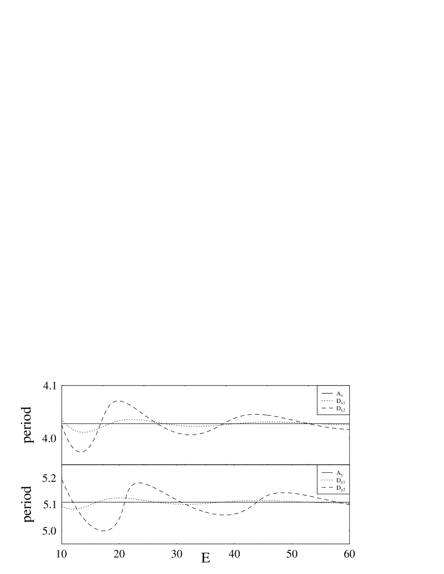
Figure 3: The periods of the $A^{\pm}$ and $D^{\pm}$ orbits as functions of energy for $\tilde{\kappa}=0.67$. The periods are given in units of $1/\Omega_{0}$, the energy unit is $2S\Omega_{0}$. For the orbits $A_{x}^{\pm}$ and $A_{y}^{\pm}$ the periods are independent of energy and equal to $\tilde{T}_{1}\approx 4.02768$ and $\tilde{T}_{2}\approx 5.10828$, respectively.

The spin-orbit strength $\tilde{\kappa}$ depends on the band structure [11]. For example, for an InGaAs-InAlAs quantum dot with $\sim 100$ confined electrons one would obtain a value of $\tilde{\kappa}\sim 0.25$. In order to have the effect of spin on the orbital motion more pronounced, we choose $\tilde{\kappa}=0.67$ for our numerics.

The stability determinant in the trace formula can be calculated according to the general prescription (Sec. 4.3). The second variation of the Hamiltonian (95) is

$$\tilde{\cal H}^{(2)} = \frac{\tilde{\rho}_{1}^{2}}{2}+\frac{\tilde{\rho}_{2}^{2}}{2}+\frac{\omega_{1}^{2}\tilde{\lambda}_{1}^{2}}{2}+\frac{\omega_{2}^{2}\tilde{\lambda}_{2}^{2}}{2}$$ (105)

$$+ \tilde{\kappa}(u\tilde{p}_{2}-v\tilde{p}_{1})(\xi^{2}+\nu^{2})+\tilde{\kappa}\frac{2\sqrt{2}\,uv}{1+u^{2}+v^{2}}(\tilde{\rho}_{2}\nu-\tilde{\rho}_{1}\xi)$$

$$+ \tilde{\kappa}\sqrt{2}\left(\frac{2u^{2}}{1+u^{2}+v^{2}}-1\right)\tilde{\rho}_{2}\xi-\tilde{\kappa}\sqrt{2}\left(\frac{2v^{2}}{1+u^{2}+v^{2}}-1\right)\tilde{\rho}_{1}\nu,$$

where the variables $\lambda$ and $\rho$ are scaled like $\bf q$ and $\bf p$, respectively. Numerically solving the equations of motion for variations

$$\dot{\tilde{\lambda}}_{1} = \tilde{\rho}_{1}-\tilde{\kappa}\sqrt{2}\frac{2uv}{1+u^{2}+v^{2}}\xi-\tilde{\kappa}\sqrt{2}\left(\frac{2v^{2}}{1+u^{2}+v^{2}}-1\right)\nu,$$ (106)

$$\dot{\tilde{\lambda}}_{2} = \tilde{\rho}_{2}+\tilde{\kappa}\sqrt{2}\left(\frac{2u^{2}}{1+u^{2}+v^{2}}-1\right)\xi+\tilde{\kappa}\sqrt{2}\frac{2uv}{1+u^{2}+v^{2}}\nu,$$ (107)

$$\dot{\nu} = -\tilde{\kappa}\frac{2\sqrt{2}\,uv}{1+u^{2}+v^{2}}\tilde{\rho}_{1}+\tilde{\kappa}\sqrt{2}\left(\frac{2u^{2}}{1+u^{2}+v^{2}}-1\right)\tilde{\rho}_{2}+2\tilde{\kappa}(u\tilde{p}_{2}-v\tilde{p}_{1})\xi,$$ (108)

$$\dot{\tilde{\rho}}_{1} = -\omega_{1}^{2}\tilde{\lambda}_{1},$$ (109)

$$\dot{\tilde{\rho}}_{2} = -\omega_{2}^{2}\tilde{\lambda}_{2},$$ (110)

$$\dot{\xi} = \tilde{\kappa}\sqrt{2}\left(\frac{2v^{2}}{1+u^{2}+v^{2}}-1\right)\tilde{\rho}_{1}-\tilde{\kappa}\frac{2\sqrt{2}\,uv}{1+u^{2}+v^{2}}\tilde{\rho}_{2}-2\tilde{\kappa}(u\tilde{p}_{2}-v\tilde{p}_{1})\nu,$$ (111)

one determines the reduced monodromy matrix and then finds the stability determinant $\det(\widetilde{M}_{po}-I_{4})$ of the periodic orbits.

After calculating the Maslov indices within Sugita’s approach [32] and the Solari-Kochetov phase by (52), we can compute the oscillating part of the density of states using the trace formula (55) (Fig. 4). Note that while the classical dynamics in the scaled variables is independent of the value of spin, the density of states will depend on $S$, since the unscaled action $2S\tilde{\mathcal{S}}$ enters the phase of the trace formula. We choose the physically meaningful $S=\hbar/2$ in our example. To ensure the convergence of the periodic orbit sum, the density of states was convoluted with a normalized Gaussian, $\exp[-(E/\gamma)^{2}]/\gamma\sqrt{\pi}$, i.e., it was smoothed out with the energy window $\sim\gamma$. With the averaging parameter $\gamma=0.6$, the first repetitions of the 12 primitive periodic orbits $A$ and $D$ were sufficient in the trace formula. The semiclassical result for the density of states is compared with the quantum-mechanical curve, obtained from a numerical diagonalization of the Hamiltonian (83). We observe a rather good agreement between the two, especially for the oscillation frequencies. The difference in the amplitudes can be explained by the vicinity of the bifurcations in the parameter space. Indeed, the disparity becomes larger near the avoided bifurcations, where the stabilities are extremely small (Fig. 4). In principle, these energy regions should be treated by a uniform approximation [29]. The matter is complicated, however, by the fact that the avoided bifurcations are non-generic and of codimension larger than 1. The theory for such bifurcations is developed only for two-dimensional systems. Our system is effectively three-dimensional. In addition to the elliptic and (inverse) hyperbolic orbits, it also has the loxodromic orbits. Thus, the extension of the standard theory of bifurcations is difficult and still needs to be developed.

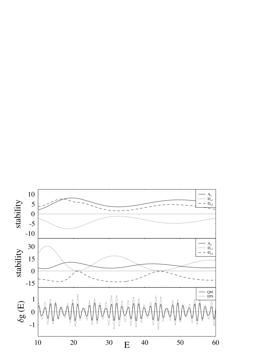
Figure 4: Upper and middle panels: the stabilities $\det(\widetilde{M}_{po}-I_{4})$ of the $A^{\pm}$ and $D^{\pm}$ orbits. The curves come close to the zero level, but do not touch or cross it (avoided bifurcations). Lower panel: the oscillating part of density of states for $\tilde{\kappa}=0.67$ and $S=\hbar/2$. QM: the quantum-mechanical direct diagonalization. EPS: the semiclassical calculation in the extended phase space, including only the first repetitions of the 12 primitive periodic orbits $A$ and $D$ (Gaussian averaging parameter $\gamma=0.6$). The energy is measured in units of $\hbar\Omega_{0}$.

A more detailed view of $\delta g(E)$ is shown in Fig. 5. For comparison, we added there the density of states calculated by the WCL trace formula with spin $S=\hbar/2$, which, in this case, is the trace formula of the two-dimensional anisotropic harmonic oscillator without spin-orbit coupling [6] multiplied by the spin degeneracy factor 2 (see above). Clearly, it is shifted by phase from the exact density of states. It is worth mentioning that the dashed (WCL) curve would come very close to the exact quantum-mechanical curve if the former is shifted by $-\tilde{\kappa}^{2}/2$ in the scaled energy $\tilde{E}$. Note that the action of the trivial periodic orbits is $\tilde{\mathcal{S}}_{i}=(\pi/\omega_{i})(2\tilde{E}+\tilde{\kappa}^{2})$. Thus the shift can be related to the perturbative correction to the action in the extended phase space, which is of the second order in $\tilde{\kappa}$. To explain the shift, it would be interesting to develop the second-order perturbation theory in the parameter $\tilde{\kappa}$ for the trace formula in the extended phase space, similar to that proposed in [7]. (The first-order perturbation theory [9] should be equivalent to the WCL trace formula.) Apparently, the shift of the dashed curve cannot be justified within the standard WCL approach of [5]. With the increase of $\tilde{\kappa}$, the non-integrability of the system will show up, and the shape of the WCL curve (describing the integrable system) will start to deviate from the exact density of states.

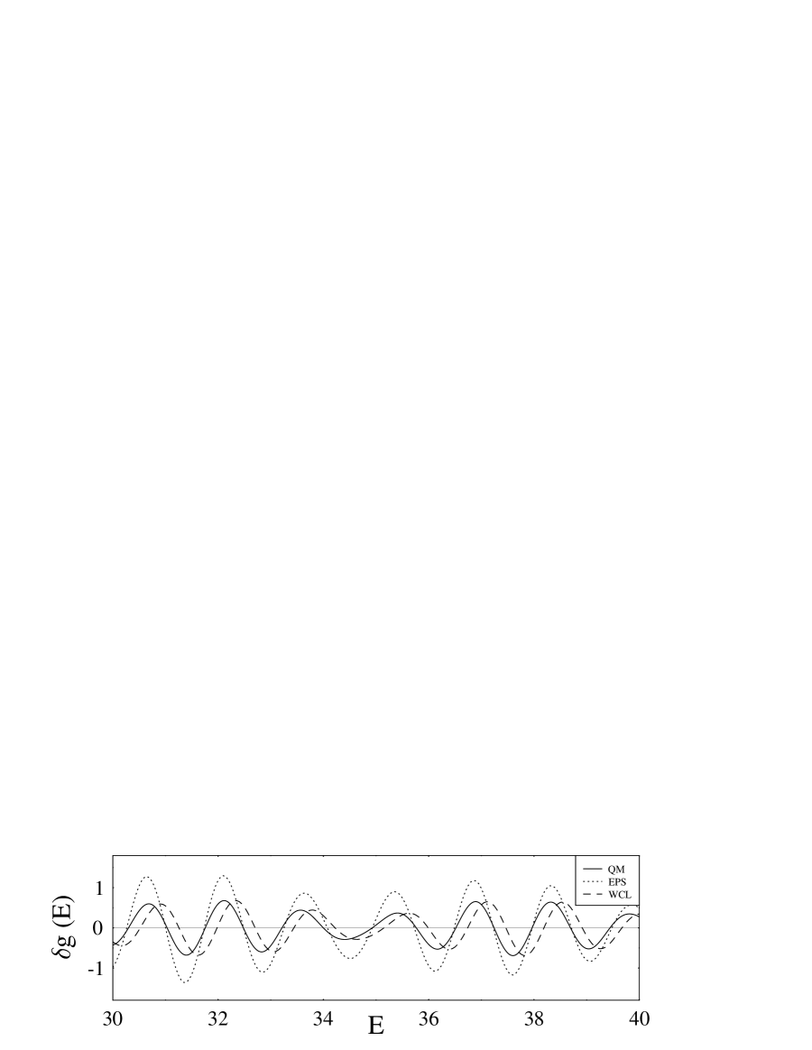
Figure 5: A detailed view of the lower panel of Fig. 4 with the WCL density of states added.

6 Conclusion

We have presented a detailed discussion of a new semiclassical method for systems with spin-orbit coupling. The key idea of this approach is to introduce an extended phase space of orbital and spin degrees of freedom where the semiclassical dynamics takes place. The recipe for the construction of such a phase space, as well as the equations of motion there, can be obtained from the path-integral formulation of quantum mechanics using the spin coherent states, with a subsequent stationary-phase evaluation.

We have classified the possible regimes according to the strength of the spin-orbit coupling and the value of the spin. When the Hamiltonian is linear in the spin, our method works not only in the standard semiclassical domain of large spin, but also for any finite spin. From the path-integral formulation we have directly derived the trace formulae in the limiting cases of weak and (under certain restriction) strong spin-orbit coupling for arbitrary spin. It was argued that the semiclassical approach in the extended phase space recovers the limiting behavior.

The general method was illustrated with the specific examples relevant, in particular, to the mesoscopic physics of heterostructures. Our analytical and numerical results underscore the importance of the Solari-Kochetov phase correction in the coherent-state path integrals and the proper evaluation of the Maslov indices in the extended phase space.

The future work in this direction might include the improvement of the semiclassical evaluation of path integrals in the case of strong spin-orbit coupling (restoration of the no-name term); generalizations of the method treating symmetry breaking and bifurcations by uniform approximations; study of models with the Hamiltonian nonlinear in spin and driven by an external system, such as the kicked top [16]; and further applications to specific systems of interest in spintronics, molecular dynamics, and nuclear physics.

Appendix A Exact quantum-mechanical evaluation of the modulation factor (27)

A.1 Exact calculation of the trace of a spin propagator

We consider a spin in the external magnetic field ${\bf C}(t)\equiv(2{\rm Re}\,f(t),-2{\rm Im}\,f(t),2A(t))$ described by the Hamiltonian

$$\mathcal{H}(t)=\hbar\,\hat{\mathbf{s}}\cdot\mathbf{C}(t)=\hbar\,[2A(t)\hat{s}_{3}+f(t)\hat{s}_{+}+(f(t))^{*}\hat{s}_{-}].$$ (112)

Its exact quantum-mechanical propagator between the spin coherent states $|z_{i}\rangle$ and $\langle z_{f}|$ is [22]

$$K_{s}(z_{f}^{*},z_{i};T)=\frac{[a^{*}(T)-b^{*}(T)\,z_{i}+b(T)z^{*}_{f}+a(T)\,z^{*}_{f}z_{i}]^{2s}}{(1+|z_{f}|^{2})^{s}(1+|z_{i}|^{2})^{s}}$$ (113)

where the coefficients $a(T)$, $b(T)$ are to be found from the equation

$$\frac{d}{dt}\left(\begin{array}[]{cc}a&b\\ -b^{*}&a^{*}\end{array}\right)=-i\left(\begin{array}[]{cc}A&f\\ f^{*}&-A\end{array}\right)\left(\begin{array}[]{cc}a&b\\ -b^{*}&a^{*}\end{array}\right)$$ (114)

with the initial conditions $a(0)=1$, $b(0)=0$. One can observe that the determinant of the matrix

$$U(t)=\left(\begin{array}[]{cc}a(t)&b(t)\\ -b^{*}(t)&a^{*}(t)\end{array}\right)$$ (115)

remains constant: $|a(t)|^{2}+|b(t)|^{2}=1$. Hence, $U(t)$ belongs to the group SU(2) and can be represented in the form

$$U(t)=\cos\frac{\eta(t)}{2}+i({\bf m}(t)\cdot\mbox{{\boldmath$\sigma$ \unboldmath}}\!\!)\sin\frac{\eta(t)}{2},$$ (116)

where ${\bf m}^{2}=1$ and $\sigma$ is a vector of Pauli matrices. Comparing (115) and (116) we deduce that

$$a(t)=\cos\frac{\eta(t)}{2}+im_{3}(t)\,\sin\frac{\eta(t)}{2},\quad b(t)=i[m_{1}(t)-im_{2}(t)]\sin\frac{\eta(t)}{2}.$$ (117)

Since

$$\frac{1}{2}{\bf C}(t)\cdot\mbox{{\boldmath$\sigma$ \unboldmath}}\!\!=\left(\begin{array}[]{cc}A(t)&f(t)\\ f^{*}(t)&-A(t)\end{array}\right),$$ (118)

we can rewrite (114) as

$$\frac{d}{dt}U(t)=-\frac{i}{2}({\bf C}(t)\cdot\mbox{{\boldmath$\sigma$ \unboldmath}}\!\!)U(t),\quad U(0)=I_{2}.$$ (119)

Note that this equation has the same form as the equation for a spin-1/2 propagator in the standard $|s,m_{s}\rangle$ basis.

The trace of the spin propagator (113) is

$$Z_{s}(T)={\rm Tr}\,K_{s}=\int d\mu_{s}(z^{\prime*},z^{\prime})\,K_{s}(z_{f}^{*}=z^{\prime*},z_{i}=z^{\prime};T),$$ (120)

where $d\mu_{s}(z^{\prime*},z^{\prime})$ is given by (16) and

$$K_{s}(z^{\prime*},z^{\prime};T)=\left[\frac{a^{*}(T)-b^{*}(T)z^{\prime}+b(T)z^{\prime*}+a(T)|z^{\prime}|^{2}}{1+|z^{\prime}|^{2}}\right]^{2s}.$$ (121)

After the stereographic projection [cf. (22)]

$$n^{\prime}_{1}+in^{\prime}_{2}\equiv\sin\theta^{\prime}\exp(i\phi^{\prime})=\frac{2z^{\prime*}}{1+|z^{\prime}|^{2}},\quad n^{\prime}_{3}\equiv\cos\theta^{\prime}=-\frac{1-|z^{\prime}|^{2}}{1+|z^{\prime}|^{2}}$$ (122)

and simple transformations we can cast (121) into the form

$$K_{s}({\bf n^{\prime}};T)=\left(\cos\frac{\eta(T)}{2}+i{\bf n^{\prime}}\cdot{\bf m}(T)\sin\frac{\eta(T)}{2}\right)^{2s}.$$ (123)

Since the measure

$$d\mu_{s}(z^{\prime*},z^{\prime})=d\mu_{s}({\bf n^{\prime}})=\frac{2s+1}{4\pi}\sin\theta^{\prime}\,d\theta^{\prime}\,d\phi^{\prime}$$ (124)

is invariant under rotations, we can choose the axis $\mathbf{e}_{3}$ along ${\bf m}(T)$. Then

$$Z_{s}(T)=\int d\mu_{s}({\bf n^{\prime}})K_{s}({\bf n^{\prime}};T)=\int d\mu_{s}({\bf n^{\prime}})\left(\cos\frac{\eta(T)}{2}+in^{\prime}_{3}\sin\frac{\eta(T)}{2}\right)^{2s}.$$ (125)

Making the following transformations in (125)

$$Z_{s}(T) = \frac{2s+1}{2}\int_{0}^{\pi}\left(\cos\frac{\eta(T)}{2}+i\cos\theta^{\prime}\sin\frac{\eta(T)}{2}\right)^{2s}\sin\theta^{\prime}d\theta^{\prime}$$

$$= \frac{2s+1}{2}\int_{-1}^{1}\left(\cos\frac{\eta(T)}{2}+ix\sin\frac{\eta(T)}{2}\right)^{2s}dx$$

$$= \frac{1}{2i\sin[\eta(T)/2]}\left(\cos\frac{\eta(T)}{2}+ix\sin\frac{\eta(T)}{2}\right)^{2s+1}\bigg{|}^{x=1}_{x=-1},$$

we obtain the final result

$$Z_{s}(T)=\frac{\sin[(s+1/2)\eta(T)]}{\sin[\eta(T)/2]},$$ (126)

where $\eta(T)$ is found from $2\cos[\eta(T)/2]=2{\rm Re}[a(T)]\equiv{\rm Tr}[U(T)]$.

In order to give the geometric interpretation of $\eta(T)$, consider an equation for the spin $s$ propagator [cf. (119)]

$$\frac{d}{dt}{\cal D}^{s}=-i({\bf C}\cdot{\bf J}^{s}){\cal D}^{s},\quad{\cal D}^{s}(0)=I_{2s+1},$$ (127)

where ${\bf J}^{s}=(J_{1}^{s},J_{2}^{s},J_{3}^{s})$ are the generators of the $(2s+1)$-dimensional irreducible representation of SU(2). Since ${\cal D}^{s}(T)=\exp[i{\bf m}(T)\cdot{\bf J}^{s}\eta(T)]$, as well as $U(T)=\exp[i{\bf m}(T)\cdot\mbox{{\boldmath$\sigma$ \unboldmath}}\!\!\eta(T)/2]$, $\eta(T)$ has the meaning of the rotation angle around the ${\bf m}(T)$ axis.

Note that one can alternatively find $Z_{s}(T)$ as ${\rm Tr}[{\cal D}^{s}(T)]$. Choosing ${\bf m}(T)$ as a quantization axis and making simple calculations, one would obtain the result coinciding with (126).

A.2 Calculation of $\eta(T)$

For the reader’s convenience we derive (31) within our notation. We will closely follow the discussion in [5], where this result previously appeared.

Without loss of generality we can choose the basis in which ${\bf e}_{3}={\bf m}(T)$. One can decompose $U(t)$ (115) at every $t$ into the matrix product

$$U(t)=\left(\begin{array}[]{cc}\cos(\theta/2)\,e^{-i\phi}&-\sin(\theta/2)\\ \sin(\theta/2)&\cos(\theta/2)\,e^{i\phi}\end{array}\right)\left(\begin{array}[]{cc}e^{i\psi}&0\\ 0&e^{-i\psi}\end{array}\right)\equiv U_{1}(t)U_{0}(t),$$ (128)

where $a=\cos(\theta/2)\,e^{i(\psi-\phi)}$ and $b=-\sin(\theta/2)\,e^{-i\psi}$. Decomposition (128) corresponds to the choice of a certain section in the principal U(1) Hopf bundle over $\mathbb{S}^{2}$, $\psi$ being a fiber coordinate. Imposing the time periodicity on $U_{1}(t)$ and recalling that $U(0)=I_{2}$, we establish that

$$\psi(T)-\psi(0)=\eta(T)/2.$$ (129)

Note that the decomposition (128) is not well defined at $t=0$, i.e., when $\theta=0$. Hence, the initial value $\psi(0)$ is not determined. (Still, $\eta(T)$ can be found unambiguously.) Although not essential for our purposes, the problem can be fixed if we choose a different decomposition near $\theta=0$, related to the former by a gauge transformation [5, 35].

We define the projection of the Hopf bundle $(\theta,\phi,\psi)\in\mathbb{S}^{3}\longrightarrow{\bf n}\in\mathbb{S}^{2}$ by

$${\bf n}\cdot\mbox{{\boldmath$\sigma$ \unboldmath}}\!\!=U\sigma_{3}U^{{\dagger}}=U_{1}\sigma_{3}U_{1}^{{\dagger}},$$ (130)

which is equivalent to $n_{1}+in_{2}=\sin\theta\exp(i\phi)$, $n_{3}=\cos\theta$. One can find equations for ${\bf n}(t)$ and $\psi(t)$ from (119). Thus, one should calculate

$$\dot{{\bf n}}=\frac{1}{2}{\rm Tr}\left[\mbox{{\boldmath$\sigma$ \unboldmath}}\!\!\frac{d}{dt}\left(U\sigma_{3}U^{{\dagger}}\right)\right]$$ (131)

to recover the equation

$$\dot{{\bf n}}={\bf C}\times{\bf n},\quad{\bf n}(0)={\bf n}(T).$$ (132)

After the stereographic projection (22) it becomes

$$\dot{z}=-i[2Az+f-f^{*}z^{2}],\quad z(0)=z(T).$$ (133)

To derive an equation for $\psi$ one should calculate

$$\dot{\psi}-\frac{1}{2}(1+\cos\theta)\dot{\phi}=-\frac{i}{2}{\rm Tr}\left[\sigma_{3}U^{{\dagger}}\frac{d}{dt}U\right]$$ (134)

taking into account (128) and (133). In the language of the fiber bundle theory, it corresponds to the pull-back of the canonical connection form [r.h.s. of (134)] onto the section defined by (128). The result of the calculation is

$$\dot{\psi}=\frac{1}{2i}\frac{z\dot{z}^{*}-z^{*}\dot{z}}{1+|z|^{2}}-\frac{1}{2}{\bf C}\cdot{\bf n}(z^{*},z)=[A-(f^{*}z+fz^{*})/2].$$ (135)

Integrating it we find

$$\eta(T) = 2[\psi(T)-\psi(0)]=\int_{0}^{T}dt\left[\frac{z\dot{z}^{*}-z^{*}\dot{z}}{i(1+|z|^{2})}-{\bf C}\cdot{\bf n}(z^{*},z)\right]$$ (136)

$$= \int_{0}^{T}dt\,[2A-(f^{*}z+fz^{*})],$$

where $z(t)$ and $z^{*}(t)$ are to be found from (133).

Appendix B Adiabatic limit in the extended phase space

Here we present an intuitive derivation of the trace formula (41) within the framework of our semiclassical theory in the extended phase space (Sec. 4.3). In the adiabatic regime the classical system, described by the Hamiltonian $\mathcal{H}$ (21), possesses an adiabatic invariant—the angle $\beta$ between the instantaneous magnetic field $\mathbf{C}$ and the classical spin vector $\mathbf{n}$. To demonstrate this, let us consider the quantity $\alpha\equiv\cos\beta=\mathbf{n}\cdot\mathbf{n}_{C}$, where $\mathbf{n}_{C}\equiv\mathbf{C}/|\mathbf{C}|$ (Fig. 6). Its time derivative averaged over the fast spin motion is

$$\left<\dot{\alpha}\right>=\left<\mathbf{n}\cdot\dot{\mathbf{n}}_{C}\right>\approx 0$$ (137)

taking into account that $\dot{\mathbf{n}},\;\dot{\mathbf{n}}_{C}\perp\mathbf{n}_{C}$.

Figure 6: Classical spin precessing about the instantaneous magnetic field.

Having an approximate integral of motion $\alpha$ has two consequences. First, the fast spin precession about $\mathbf{C}$ can be separated from the orbital motion in the adiabatic limit. The latter then is described by the polarized Hamiltonian

$$\mathcal{H}_{\alpha}({\bf q,p})=\mathcal{H}_{0}({\bf q,p})+\hbar s\alpha|{\bf C}({\bf q},{\bf p})|$$ (138)

with $\alpha$ as a parameter. Second, in a system with one integral of motion in addition to the energy, the periodic orbits are not isolated, but appear in one-parameter families instead. Hence, we should use the modified trace formula [10] that involves the summation over the periodic orbit families (p.o.f.):

$$\delta g_{sc}(E)=-\mathrm{Im}\,\frac{1}{i\pi\hbar}\sum_{\mathrm{p.o.f.}}\left[\frac{2\pi}{(2\pi i\hbar)^{1/2}\left|\frac{\partial\eta}{\partial J}\right|^{1/2}}\right]\frac{T_{ppo}\exp\left(\frac{i}{\hbar}{\cal S}+i\varphi^{SK}-i\frac{\pi}{2}\sigma\right)}{\left|\det\left(\widetilde{M}_{\mathrm{orb}}-I_{2(d-1)}\right)\right|^{1/2}},$$ (139)

where the factor in the square brackets is absent in the standard Gutzwiller trace formula for isolated orbits, the stability matrix $\widetilde{M}_{\mathrm{orb}}$ is calculated only for the orbital subspace, the action ${\cal S}$, Solari-Kochetov phase $\varphi^{SK}$, and Maslov index $\sigma$ are evaluated for any representative of a family. $J=\hbar s\alpha$ is the classical-spin projection on the direction $\mathbf{n}_{C}$ of the field and

$$\eta(\alpha)\equiv\eta[\mathbf{q,p};T_{po}^{(\alpha)}]$$ (140)

is the total angle of rotation of the Bloch sphere for a periodic orbit of $\mathcal{H}_{\alpha}$, where the r.h.s. of (140) is calculated according to (36) (cf. Sec. 4.1 and Ref. [36]). Obviously, we have $\eta\gg 2\pi$, since the spin vector makes many rotations during the period of the orbital motion.

As a result of the approximate separation of variables, to any classical trajectory of $\mathcal{H}_{\alpha}({\bf q,p})=E$ corresponds a family of classical trajectories in the extended phase space. This family will consist of periodic orbits if the respective orbit of $\mathcal{H}_{\alpha}$ is periodic and the Bloch sphere makes an integer number of rotations during the orbital period. The latter condition follows from the fact that the whole family, not just an isolated orbit, is periodic on the Bloch sphere. Thus, we have a requirement

$$\eta(\alpha)=2\pi N(\alpha)\quad(N(\alpha)\gg 1)$$ (141)

with an integer $N(\alpha)$. Clearly, this condition can be satisfied only for selected values of $\alpha$. Now we will show that the allowed values of $\alpha$ form discrete sets that become very dense in the adiabatic limit. Consider a periodic orbit of $\mathcal{H}_{\alpha=-1}$. Let us assume that as $\alpha$ changes from $-1$ to $1$ for fixed energy, the orbit can be continuously deformed while maintaining its periodicity and that $\eta(\alpha)$ increases with $\alpha$. If for $\alpha=-1$ the requirement (141) is not fulfilled, we shift $\alpha$ by a small amount to $\alpha=\alpha_{0}$, such that $\eta(\alpha_{0})=2\pi N$. The greater the frequency of precession $|{\bf C}|$, the smaller the shift. Changing $\alpha$ further to $\alpha_{1}>\alpha_{0}$, we achieve that the Bloch sphere makes one more rotation for the newly deformed orbit, i.e., $\eta(\alpha_{1})=2\pi(N+1)$. We continue this process till we reach the upper bound $\alpha_{L}\leq 1$ for which $\eta(\alpha_{L})=2\pi(N+L)$. Thus, we have constructed a set $\{-1\leq\alpha_{0}<\alpha_{1}<\ldots<\alpha_{L}\leq 1\}$ of the values of $\alpha$ for which the families of orbits in the extended phase space are periodic. We will call it the periodic-orbit set (p.o.s.). The better the adiabaticity condition (33) is fulfilled, the larger the number of elements of the p.o.s. $L\gg 1$. The periodic orbits within the set are related by an almost continuous transformation in the $({\bf q,p})$ space (Fig. 7). If we start with a different periodic orbit of $\mathcal{H}_{\alpha=-1}$, we will obtain another p.o.s. The sum over the p.o.f. in (139) can be represented as the sum over all sets and the elements within each set, i.e.,

$$\sum_{\mathrm{p.o.f.}}\,(\ldots)=\sum_{\mathrm{p.o.s.}}\,\sum_{n=N}^{N+L}\,(\ldots)=\sum_{\mathrm{p.o.s.}}\,\sum_{M=-\infty}^{\infty}\int_{N}^{N+L}dn\,e^{2\pi iMn}\,(\ldots).$$ (142)

In the second equality we applied the Poisson summation formula to the inner sum.

Figure 7: Elements of the periodic orbit set in the orbital subspace.

Our conclusions may seem to disagree with the results of Sec. 4.2, where we have found for the periodic orbits in the extended phase space that $\alpha\approx\pm 1$. There is no contradiction, however, if we recall that in (37) the magnetic field $\mathbf{C}$ was predetermined, so that, in general, the orbital frequency and the overall frequency of precession were incommensurate. Therefore the spin must have been aligned with the field in order to have a periodicity in the extended phase space. In the present case, on the other hand, there is a feedback from the spin to the orbital degrees of freedom, and for certain initial conditions the frequencies become commensurate, thus producing the periodic-orbit sets.

We now turn to the calculation of the action which can be divided into the orbital and spin parts [cf. (49)]. The orbital part $\mathcal{S}_{\mathrm{orb}}^{(\alpha)}$ is evaluated in the usual way with the Hamiltonian $\mathcal{H}_{\alpha}({\bf q,p})=E$. The spin part is given in terms of the spin orientation $\mathbf{n}(\theta,\phi)$ by

$$\mathcal{S}_{\mathrm{spin}}^{(\alpha)}=\hbar s\oint_{0}^{T_{po}^{(\alpha)}}(1+\cos\theta)\,\dot{\phi}\,dt=\hbar s[\eta(\alpha)+\alpha\Phi(\alpha)],$$ (143)

where $\Phi(\alpha)=\oint_{0}^{T_{po}^{(\alpha)}}|{\bf C}({\bf q},{\bf p})|dt$. There is a direct analogy between the problem of spin precession and the problem of a spinning top with fixed base point whose axis of rotation is moved along a closed circuit. Namely, the magnetic field orientation $\mathbf{n}_{C}(\theta_{C},\phi_{C})$ corresponds to the axis of rotation, its magnitude $|{\bf C}|$ becomes the angular velocity of rotation, and the spin orientation $\mathbf{n}(\theta,\phi)$ is a direction on the top making angle $\beta$ with the axis (Fig. 8). Then the standard theory of adiabatic motion [17] provides the relation

$$\eta(\alpha)-4\pi=\Phi(\alpha)-\Omega(\alpha),$$ (144)

where $\Omega(\alpha)=\oint_{0}^{T_{po}^{(\alpha)}}(1+\cos\theta_{C})\,\dot{\phi}_{C}\,dt$ is the solid angle swept over by the axis of rotation in the lower hemisphere during the period. Using (144) in (143) and taking into account (141), we obtain the spin action

$$\mathcal{S}_{\mathrm{spin}}^{(\alpha)}-4\pi\hbar s=2\pi\hbar s\,(\alpha+1)N(\alpha)+\hbar s\alpha\Omega(\alpha),$$ (145)

where $N(\alpha)$ was shifted by $-2$. The second term on the right is the origin of the Berry phase.

Figure 8: Illustration of the coordinates’ notation. $\Phi(t)=\int_{0}^{t}|{\bf C}({\bf q},{\bf p})|dt$.

The Solari-Kochetov phase $\varphi^{SK}_{\alpha}=\eta(\alpha)/2=\pi N(\alpha)$ is equal to an integer multiple of $\pi$. We expect that together with the Maslov index $\sigma$, it will yield, at the end of the calculation, the usual Maslov index $\sigma_{po}^{(\alpha)}$ for the trace formula of the Hamiltonian $\mathcal{H}_{\alpha}({\bf q,p})$ in the orbital subspace. However, at this point we have not succeeded in establishing this connection.

We can do the summation over the p.o.f. in the trace formula (139) with the help of (142), where the integral can be computed by stationary phase. For this we express all $\alpha$-dependent quantities in terms of $N(\alpha)$ and then substitute it by a continuous variable $n$. Only $\mathcal{S}_{\mathrm{orb}}^{(\alpha)}$ and $2\pi\hbar s(\alpha+1)N(\alpha)$ determine the stationary-phase point, the remaining functions are slowly varying with $n$. The stationary-phase condition is

$$0=2\pi M+\frac{1}{\hbar}\frac{\partial}{\partial n}\left(\mathcal{S}_{\mathrm{orb}}^{(\alpha)}+2\pi\hbar s[\alpha(n)+1]n\right)=2\pi M+2\pi s[\alpha(n)+1],$$ (146)

where the result of the classical perturbation theory

$$\frac{\partial\mathcal{S}_{\mathrm{orb}}^{(\alpha)}}{\partial\alpha}=-\oint_{0}^{T_{po}^{(\alpha)}}\frac{\partial\mathcal{H}_{\alpha}}{\partial\alpha}dt=-\hbar s\Phi(\alpha)=-2\pi\hbar sN(\alpha)+\mathcal{O}(N^{0})$$ (147)

was employed. Thus, the equation for the stationary point $\alpha\,(n_{\mathrm{st}})=-M/s-1$ has a solution only if the the r.h.s. does not exceed 1 by magnitude. This makes the $M$ sum finite, reducing it to the sum over quantized polarizations:

$$\sum_{M=-\infty}^{\infty}\int_{N}^{N+L}dn\,e^{2\pi iMn+\frac{i}{\hbar}\left(\mathcal{S}_{\mathrm{orb}}^{(\alpha)}+2\pi\hbar s[\alpha(n)+1]n\right)}\,(\ldots)$$ (148)

$$\approx\sum_{m_{s}=-s}^{s}\left\{e^{\frac{i}{\hbar}\mathcal{S}_{\mathrm{orb}}^{(\alpha)}}\,\left[\frac{(2\pi i\hbar)^{1/2}\left|\frac{\partial\eta}{\partial J}\right|^{1/2}}{2\pi}\right]\,(\ldots)\right\}_{\alpha=m_{s}/s}.$$

$m_{s}=-M-s$ is either integer or half-integer, depending on the spin $s$. It labels the quantized spin projection on the $\mathbf{n}_{C}$ axis. The prefactor due to the stationary-phase integration, that appears in the square brackets in (148), cancels the respective factor in (139). The outer sum over the p.o.s. in (142), if exchanged with the sum over $m_{s}$, becomes the sum over the periodic orbits of polarized Hamiltonians ${\cal H}_{\alpha=m_{s}/s}\mathbf{(q,p)}\equiv{\cal H}_{\mathrm{eff}}^{(m_{s})}\mathbf{(q,p)}$ (42). Thus the density of states is given by the sum of the polarized trace formulae:

$$\delta g_{sc}^{\mathrm{SCL}}(E)=\frac{1}{\pi\hbar}\sum_{m_{s}=-s}^{s}\sum_{po}\;\frac{T_{ppo}^{(m_{s})}\cos\left(\frac{S_{po}^{(m_{s})}}{\hbar}+\varphi_{B}^{(m_{s})}-\frac{\pi}{2}\sigma_{po}^{(m_{s})}\right)}{\left|\det\left(\widetilde{M}_{po}^{(m_{s})}-I_{2(d-1)}\right)\right|^{1/2}}$$ (149)

with the Berry phase

$$\varphi_{B}^{(m_{s})}=\Bigl{.}s\alpha\,\Omega(\alpha)\Bigr{|}_{\alpha=m_{s}/s}=m_{s}\oint_{0}^{T_{po}^{(m_{s})}}(1+\cos\theta_{C})\,\dot{\phi}_{C}\,dt,$$ (150)

which is equivalent to (40).

Far from being mathematically rigorous, this derivation illustrates how the sum over quantized polarizations can be obtained from the classical-spin dynamics, where any polarization is allowed. As in Sec. 4.2, the problem of the missing no-name term [25] remains here. A careful evaluation of the Maslov indices is also required.

References

- [1] A. Alscher and H. Grabert, Eur. Phys. J. D 14, 127 (2001).
- [2] Ch. Amann and M. Brack, J. Phys. A 35, 6009 (2002).
- [3] M. V. Berry and K. E. Mount, Rep. Prog. Phys. 35, 315 (1972).
- [4] See, e.g., A. Bohr and B. R. Mottelson, Nuclear Structure (W. A. Benjamin, New York, 1969), Vol. I.
- [5] J. Bolte and S. Keppeler, Phys. Rev. Lett. 81, 1987 (1998); Ann. Phys. (N.Y.) 274, 125 (1999).
- [6] M. Brack and R. K. Bhaduri, Semiclassical Physics, Frontiers in Physics Vol. 96 (Addison-Wesley, Reading, USA, 1997); revised paperback edition (Westview Press, Boulder, USA, 2003).
- [7] M. Brack, S. C. Creagh, and J. Law, Phys. Rev. A 57, 788 (1998).
- [8] Y. Bychkov and E. Rashba, J. Phys. C 17, 6039 (1984), and earlier references quoted therein.
- [9] S. C. Creagh, Ann. Phys. (N.Y.) 248, 60 (1996).
- [10] S. C. Creagh and R. G. Littlejohn, Phys. Rev. A 44, 836 (1991).
- [11] See, e.g., T. Darnhofer, M. Suhrke, and U. Rössler, Europhys. Lett. 35, 591 (1996).
- [12] S. Datta and B. Das, App. Phys. Lett. 56, 665 (1990); see also S. Das Sarma, Am. Sci. 89, 516 (2001).
- [13] H. Frisk and T. Guhr, Ann. Phys. (N.Y.) 221, 229 (1993).
- [14] T. Fukui, Progr. Theor. Phys. 87, 927 (1992).
- [15] M. C. Gutzwiller, J. Math. Phys. 12, 343 (1971).
- [16] F. Haake, Quantum Signatures of Chaos (Springer, Berlin, 1990).
- [17] J. H. Hannay, J. Phys. A: Math. Gen. 18, 221 (1985).
- [18] C.-M. Hu, J. Nitta, T. Akazaki, and H. Takayanagi, Phys. Rev. B 60, 7736 (1999); T. Matsuyama, R. Kürsten, C. Meißner, and U. Merkt, Phys. Rev. B 61, 15588 (2000).
- [19] E. T. Jaynes and F. W. Cummings, Proc. IEEE 51, 89 (1963).
- [20] S. Keppeler and R. Winkler, Phys. Rev. Lett. 88, 046401 (2002).
- [21] J. R. Klauder, Phys. Rev. D 19, 2349 (1979).
- [22] E. Kochetov, J. Math. Phys. 36, 4667 (1995).
- [23] H. Kuratsuji and T. Suzuki, J. Math. Phys. 21, 472 (1980); H. Kuratsuji and Y. Mizobuchi, J. Math. Phys. 22, 757 (1981).
- [24] See, e.g., F. Langouche, D. Roekaerts, and E. Tirapegui, Functional Integration and Semiclassical Expansions (Reidel, Dordrecht, 1982).
- [25] R. G. Littlejohn and W. G. Flynn, Phys. Rev. A 44, 5239 (1991); Phys. Rev. A 45, 7697 (1992).
- [26] M. Oestreich, Nature 402, 735 (1999); S. Das Sarma, J. Fabian, X. Hu, and I. Zutic, IEEE Trans. Magn. 36, 2821 (2000).
- [27] M. Pletyukhov, Ch. Amann, M. Mehta, and M. Brack, Phys. Rev. Lett. 89, 116601 (2002).
- [28] See, e.g., K. Richter, D. Ullmo, and R. A. Jalabert, Phys. Rep. 276, 1 (1996).
- [29] M. Sieber and H. Schomerus, J. Phys. A 31, 165 (1998), and earlier references.
- [30] H. G. Solari, J. Math. Phys. 28, 1097 (1987).
- [31] M. Stone, K.-S. Park, and A. Garg, J. Math. Phys. 41, 8025 (2000).
- [32] A. Sugita, Ann. Phys. (N.Y.) 288, 277 (2001).
- [33] M. Thoss and G. Stock, Phys. Rev. A 59, 64 (1999).
- [34] V. R. Vieira and P. D. Sacramento, Nucl. Phys. B 448, 331 (1995).
- [35] T. T. Wu and C. N. Yang, Phys. Rev. D 12, 3845 (1975).
- [36] O. Zaitsev, J. Phys. A: Math. Gen. 35, L721 (2002).