Instabilities and Bifurcations of Nonlinear Impurity Modes

Abstract

We study the structure and stability of nonlinear impurity modes in the discrete nonlinear Schrödinger equation with a single on-site nonlinear impurity emphasizing the effects of interplay between discreteness, nonlinearity and disorder. We show how the interaction of a nonlinear localized mode (a discrete soliton or discrete breather) with a repulsive impurity generates a family of stationary states near the impurity site, as well as examine both theoretical and numerical criteria for the transition between different localized states via a cascade of bifurcations.

I Introduction

Nonlinear localized modes in discrete systems, also called intrinsic localized modes or discrete breathers, are self-localized states that exist due to the interplay between lattice coupling and nonlinear effects. Spatially localized modes of the discrete nonlinear Schrödinger (DNLS) equation, known as discrete solitons, have appeared in many diverse areas of physics, such as biophysics, nonlinear optics, solid state physics [6] and, more recently, in the studies of the Bose-Einstein condensates in optical lattices [2] and photonic-crystal waveguides and circuits [3].

In application to nonlinear guided-wave optics, discrete solitons have been suggested to exist in nonlinear waveguide arrays [4], and they have been observed a decade later in AlGaAs waveguide structures [5] (see also a review paper [6]). Several other issues, such as the discreteness-induced soliton dynamics and soliton interaction, have been investigated. Regarding applications, it was recently shown that discrete solitons in two-dimensional networks of nonlinear waveguide arrays can be used to realize various functional operations, such as blocking, routing, logic functions, time gating, etc. [7].

On the other hand, localized impurities are known to play a crucial role in numerous physical systems, not only introducing interesting wave scattering phenomena [8], but also creating the possibility for the excitation of impurity modes, which are spatially localized oscillatory states at the impurity sites [9]. The relevant phenomenology has been recognized as important in a variety of physical settings ranging from defect modes in superconductors [10] to the dynamics of the electron-phonon interactions [11] and from the propagation of light in dielectric super-lattices with embedded defect layers [12] to defect modes in photonic crystals [13].

It is crucially important to examine the interplay between disorder and nonlinearity. For the continuum problems, this interplay is known to lead to the existence of symmetric and asymmetric impurity modes and their interesting stability properties (see Refs. [14, 15] and references therein). Here we concentrate on the study of the discrete systems such as the DNLS model. Some earlier results for the discrete lattices focused on the scattering of localized modes by impurities in the DNLS equation [16, 17], as well as in the Klein-Gordon model [18]. The effect of the impurity on localization properties of the nonlinear lattice and stability of localized modes was studied, to the best of our knowledge, only for lattices with anharmonic coupling [19].

However, the earlier theoretical predictions [17] and recent experimental results [20, 21] for the interaction of the discrete solitons with structural defects in arrays of AlGaAs optical waveguides suggest that discreteness should play a crucial role in the properties and stability of nonlinear localized modes. In this paper, we study, in the framework of the DNLS model, how the interaction of a discrete localized mode with a repulsive nonlinear impurity leads to different localized states, as well as examine, both analytically and numerically, the stability criteria for the bifurcations between different localized modes near the impurity site.

The existence of multiple localized states near the impurity site can be understood by means of simple physics. Indeed, in the continuum approximation, a two-hump localized mode centered at the defect [22] is known to be unstable with respect to an exponential growth of antisymmetric linear perturbations [14, 15]. The above-mentioned instability leads to the motion of the localized mode away from the defect [15], and for small distances $\xi$ between the mode center and the defect, the effective interaction energy can be presented in the form $H_{\rm int}\simeq H_{0}-A{\xi}^{2}$, where $A$ is defined by the defect parameters. However, this situation becomes quite different in discrete systems because of the so-called “Peierls relief”, an effective periodic potential due to the lattice discreteness. Such potential was first calculated for small-amplitude breathers in a nonlinear elastic chain described by the discrete nonlinear Klein-Gordon equation [23] applying an approach suggested for kinks of the Frenkel-Kontorova model [24]. The potential has the following structure, $H_{p}\simeq H_{1}-B\cos(2\pi\xi/h)$, where $h$ is the lattice spacing. Thus, a competition between these two potentials defines a sequence of stable positions of a localized mode near the defect. This qualitative picture is valid in the limit of small $h$ and, generally speaking, the problem should be solved numerically. Below, we consider this problem in the framework of the DNLS model with a single on-site nonlinear defect.

The paper is organized as follows. In Sec. II we introduce our model and discuss the analytical results obtained for the family of the stationary states localized near the defect site. Then, in Sec. III we study numerically symmetric localized modes and their symmetry-breaking instability, including the analysis of the linear eigenvalue problem. Section IV includes the results of the instability-induced dynamics of localized modes and the study of the families of asymmetric localized modes which appear as stable states due to a balance of the defect repulsion and the effective trapping potential of the lattice. We also find the families of asymmetric modes and demonstrate their stability. Finally, Sec. V concludes the paper.

II Model and Analytical Results

We consider a DNLS model with a nonlinear impurity on one site of the lattice. To examine the interplay between discreteness, nonlinearity and disorder, we study the case of a focusing nonlinearity in the waveguide array with a repulsive nonlinear defect. The DNLS equation describing our model can be written in the following dimensionless form,

$$i\dot{u}_{n}+\frac{C}{2}\Delta_{2}u_{n}+|u_{n}|^{2}u_{n}=\alpha\delta_{n,n_{0}}|u_{n}|^{4}u_{n},$$ (1)

where $\Delta_{2}u_{n}\equiv(u_{n+1}+u_{n-1}-2u_{n})$, $u_{n}$ describes the complex envelope of the electric field in the $n$-th waveguide, while the dot stands for the spatial derivative along the array propagation direction (which we treat here as time $t$).

In this study, we select the quintic nonlinearity for the defect, in order to differentiate its effect from the lattice as well as to model non-Kerr nonlinear response often observed in experiment (see, e.g. Ref. [21]). However, we expect that the results will be qualitatively valid for any type of the power-law nonlinearity of the order $n$. The generalized nonlinearity of the defect can also appear in the theory of photonic circuits [25].

The coupling coefficient $C$ can be expressed through the lattice spacing $h$ as follows $C=1/h^{2}$, and it characterizes the effective diffraction in the array. We should notice that the lattice spacing $h$ may not coincide with the relative distance between the waveguide in an array, and these values are connected in a more complicated way [26, 27].

Equation (1) stems from the Hamiltonian

$$H=\sum_{n}\frac{1}{2}\left(C|u_{n+1}-u_{n}|^{2}-|u_{n}|^{4}\right)+\frac{\alpha}{3}|u_{n_{0}}|^{6},$$ (2)

upon setting its derivative with respect to $u_{n}^{\star}$ equal to $i\dot{u}_{n}$.

The linear waves of the form $u_{n}=u_{0}\exp(i\Omega t-iknh)$ have the (phonon) spectrum $\Omega=-(2/h^{2})\sin^{2}(kh/2)$ consisting of a band of negative frequencies ($\Omega<0$).

In the homogeneous (i.e., no impurity or equivalently $\alpha=0$), continuum (i.e., $h\rightarrow 0$) limit, the model (1) has an exact localized solution of the form (in the long-wave approximation, i.e. $h\eta\ll 1$)

$$u(x,t)=\frac{\eta\;e^{i\Lambda t}}{\cosh[\eta(x-\xi)]},$$ (3)

where $\Lambda=\eta^{2}/2$, $\Lambda$ is the frequency of the breather (and should be positive to avoid resonances with the linear spectrum of plane waves), and $\eta$ essentially defines an effective mass of the breather excitation in the long wave approximation according to $M_{eff}=2\eta$.

A natural approach to the study of a discrete model is to use the expression (3) as an ansatz solution in the Hamiltonian (2) in order to obtain information about the static solution of Eq. (1) and its stability. The last term of Eq. (2) is then easy to evaluate in the framework of the ansatz (3). On the other hand, the first two terms (in the parenthesis) of Eq. (2) can be evaluated using the Poisson summation formula [28] which states that

$$\sum_{n=-\infty}^{\infty}f(\beta n)=\frac{\sqrt{2\pi}}{\beta}\sum_{m=-\infty}^{\infty}F\left(\frac{2m\pi}{\beta}\right),$$ (4)

where $F$ is the Fourier transform of $f$,

$$F(k)=\frac{1}{\sqrt{2\pi}}\int_{-\infty}^{\infty}f(x)e^{ikx}dx.$$ (5)

Using the above remarks and formulas for the Hamiltonian (2), we can evaluate $H=H(\xi;\{\eta,h\})$ (up to constant, $\xi$-independent terms) as the following

$$H=H_{p}+H_{\rm int},$$ (6)

where

$\displaystyle H_{\rm p}=-\frac{4\pi^{2}}{h^{2}}\sum_{m=1}^{\infty}\frac{m\;\cos(2m\pi\xi/h)}{\sinh(m\pi^{2}/\eta h)}\left[-\frac{1}{h^{2}}+\frac{\eta^{2}}{3}\left(1+\frac{m^{2}\pi^{2}}{\eta^{2}h^{2}}\right)\right],$

$\displaystyle H_{\rm int}=\frac{\alpha\eta^{6}}{3\,\cosh^{6}(\eta\xi)}.$

Notice that the first part of the expression pertaining to the summation assumes the correct asymptotic (i.e., small $h$) form used e.g., in Eq. (3.5) in [29], as well as in references therein. Finally, it is worth mentioning that the series in Eq. (6) has terms which are exponentially smaller with respect to the leading order terms and hence even keeping a small number of terms in the series should yield reasonably accurate results. In the leading order approximation, the Hamiltonian can be approximated as follows

$$H\simeq-\frac{16{\pi}^{2}}{h^{4}}e^{-{\pi}^{2}/h\eta}\cos(2\pi\xi/h)+\frac{\alpha{\eta}^{6}}{3\cosh^{6}\eta\xi}$$ (7)

The criterion for obtaining a steady state in the reduced variable formalism of $H=H(\xi;\{\eta,h\})$ requires that

$$\frac{\partial H}{\partial\xi}|_{\xi=0}=0.$$ (8)

It is worth noting that the fact that the solutions of Eq. (8) will be static solutions of Eq. (1) has been rigorously proved recently by Kapitula [30], through the use of a Lyapunov-Schmidt reduction. Given that the ansatz of Eq. (3) is not exact, this result should be interpreted in the orbital sense (i.e., there are orbits in the configuration space which are close to the approximate solution of Eq. (8) in conjunction with Eq. (3), in the appropriate norm). In particular, in this case one can directly observe that $\xi=0$ will always be a solution of Eq. (8). Additional solutions are present close to $\xi=nh$ ($n\in{\cal Z}$), and unstable ones close to $\xi=(n+1/2)h$. In the homogeneous limit, the pulse-like steady states are exactly at these points, as is well-known, but now the presence of the impurity modifies their exact location, albeit slightly due to the exponential decay of the impurity potential away from its location at $\xi=0$.

Of particular interest is the stability of the solution at $\xi=0$. One naturally expects that when the impurity is sufficiently strong and repulsive, it will reverse the local stability picture close to $\xi=0$, converting the relevant local energy minimum into a local energy maximum. We should note here that as per the positive definite nature of the Hessian matrix in the focusing case (for a single pulse), the local minima of the energy landscape $H=H(\xi;\{\eta,h\})$ will correspond to stable solutions. The opposite will be true for local maxima. The Hessian matrix here is given by $\partial P/\partial\Lambda$, where $P$ is the power or (squared) $L^{2}$ norm of the solution $P=||u||_{2}^{2}$ [31]. Recall that the $L^{p}$ norm is defined as $||u||_{p}=(\sum_{n}|u_{n}|^{p})^{1/p}$. The $L^{\infty}$ norm (used also below) is $||u||_{\infty}=\max_{n}|u_{n}|$. $P$ can be thought of as the number of elementary excitations present in the field. In the optics literature, this is often called the “energy” of the solution.

Hence, the instability criterion in the reduced, one degree of freedom dynamical system for the relevant steady state will be

$$\frac{\partial^{2}H}{\partial\xi^{2}}|_{\xi=0}<0,$$ (9)

which can be restated in the form of the asymptotic approximation, through the leading order term of the series in Eq. (6), as follows $\alpha>\alpha_{c}$, where

$$\alpha_{c}=\frac{32\pi^{4}}{h^{6}\eta^{8}}e^{-\frac{\pi^{2}}{\eta h}}.$$ (10)

In terms of the full series, the critical value reads

$$\alpha_{c}=\frac{8\pi^{4}}{\eta^{8}h^{6}}\sum_{m=1}^{\infty}\frac{m^{3}}{\sinh(m\pi^{2}/\eta h)}\left[-\frac{1}{h^{2}}+\frac{\eta^{2}}{3}\left(1+\frac{m^{2}\pi^{2}}{\eta^{2}h^{2}}\right)\right],$$ (11)

which can be easily confirmed to have as leading order behavior Eq. (10).

The result (11) describes the stability threshold of the discrete mode localized at the impurity site $n=0$, so that when the impurity is sufficiently strong and repulsive, it will reverse the local stability of the mode close to $\xi=0$, converting the relevant local energy minimum into a local energy maximum. However, the results (8), (9) are more general, and they suggest the existence of many different stable stationary states located at certain distances from the impurity according to the local minima of the effective energy, the minima are produced by the effective periodic potential due to the model discreteness. For all such states, the physical picture based on the reduced Hamiltonian is valid only approximately, and more detailed numerical studies are required.

III Localized modes and their stability

We now turn to numerical results. We numerically constructed solutions of Eq.(1), for the chain with $N=200$ sites, localized at the impurity site $n_{0}=100$, using a Newton method with an initial condition given by Eq. (3), assuming $\Lambda=0.5$ ($\eta=1$). Upon convergence, linear stability analysis of the resulting pulses was performed. This was done by linearizing using the ansatz: $u_{n}=u_{sol}+\epsilon\exp(i\Lambda t)[a_{n}\exp(-i\omega t)+b_{n}\exp(i\omega^{*}t)]$; $u_{sol}$ is the exact solution (around which we are linearizing) and the $\omega$’s denote the linearization eigenfrequencies. Then to O($\epsilon$) we obtain the relevant (linearization) eigenvalue problem

$\displaystyle\omega\left(\begin{array}[]{c}a_{k}\\ b_{k}^{\star}\\ \end{array}\right)={\bf J}\cdot\left(\begin{array}[]{c}a_{k}\\ b_{k}^{\star}\\ \end{array}\right),\\$

where ${\bf J}$ is the linear stability (Jacobian) matrix of the form

$\displaystyle{\bf J}=\left(\begin{array}[]{cc}\frac{\partial{F_{i}}}{\partial u_{j}}&\frac{\partial{F_{i}}}{\partial u_{j}^{\star}}\\ -\frac{\partial{F_{i}^{\star}}}{\partial u_{j}}&-\frac{\partial{F_{i}^{\star}}}{\partial u_{j}^{\star}}\\ \end{array}\right),\\$

where $F_{i}=-\frac{1}{2}C(u_{i+1}+u_{i-1}-2u_{i})-u_{i}^{2}u_{i}^{\star}+\alpha u_{i}^{3}{u_{i}^{\star}}^{2}\delta_{i,n_{0}}$. When the corresponding eigenfrequencies $\omega$ are real, then the solution is linearly stable. On the contrary, the presence of a mode with a nonzero imaginary part in its eigenfrequency denotes the presence of an instability.

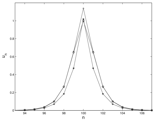
FIG. 1.: Nonlinear localized mode in the model (1) for $h=1$. Solid line with circles depicts the continuum solution (3). Stars and pluses denote the discrete solution ($h=1$) at $\alpha=0$ and $\alpha=\alpha_{c}\approx 0.22$, respectively. In the discrete case, the solid line is a guide for eye only.

Figure 1 shows a typical mode profile obtained in different cases. These soliton profiles are similar to those discussed in the long-wave approximation in Refs. [14, 15, 22]. For $\alpha=0$ (homogeneous case), the circles denote the discretization of the continuum profile in accordance with Eq. (3). The corresponding exact discrete homogeneous solution is shown by the stars. These results are shown for the lattice spacing parameter $h=1$. Notice, that discreteness induces a narrowing and increase of amplitude with respect to the continuum pulse. Finally, the pluses indicate the solution at the onset of the instability (that occurs as $\alpha$ is increased), for $\alpha=0.22$. An interesting observation is that at the onset of the instability, the pulse has essentially regained its continuum shape but for a significantly larger amplitude at the central site.

A more detailed study of the mode instability that occurs as $\alpha$ is increased is presented in Figs. 2 and 3. Figure 2 shows three different examples of the discrete localized mode and the corresponding linear stability results. The top panel is for $\alpha=0.1$, in the subcritical case, where the stability of the mode can be determined by the absence of imaginary eigenfrequencies (see the top right panel in Fig. 2). The middle row shows a slightly supercritical value of the impurity strength ($\alpha=0.3$, while $\alpha_{c}\approx 0.22$), while a strongly unstable, supercritical mode for $\alpha=0.5$ is shown in the bottom panel. It is important to remark here that a perhaps counter-intuitive result of our numerical investigations is that the instability point is not coincident with the point (in parameter space) where the symmetric mode becomes two-humped. We have generically observed that the mode becomes two-humped for considerably larger (than the instability threshold) values of the defect strength $\alpha$.

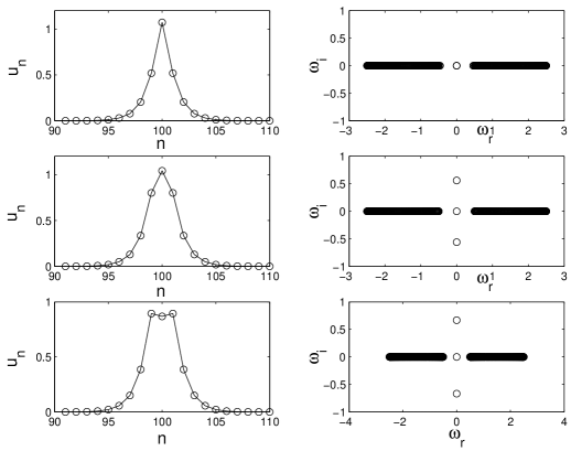
FIG. 2.: Different localized modes (left panels) and their stability properties (right panels) in the model (1) for $h=1$. Results of the linear stability analysis are given in the form of the spectral plane $(\omega_{r},\omega_{i})$ showing the real and imaginary part of the eigenfrequency, respectively. The top row is for $\alpha=0$, the middle is for $\alpha=0.3>\alpha_{c}$, while the bottom is for $\alpha=0.5$.

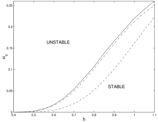
FIG. 3.: Threshold of the instability onset for the nonlinear impurity mode centered at the impurity site, shown as the critical impurity strength $\alpha_{c}$ vs. the lattice spacing $h$. Solid line–the full numerical result, dashed line is given by Eq. (10), the dash-dotted is given by Eq. (11).

Similar calculations were performed for different values of the discreteness parameter $h$ and a two-parameter stability diagram is shown in Fig. 3. Above the different curves the (centered at $\xi=0$) solutions are unstable, while the opposite is true below the curves. The solid line denotes the exact numerical result, the dashed line is the prediction of Eq. (10), while the dash-dotted line is the prediction of Eq. (11) including $m=50$ terms in the summation. One can observe that even though the asymptotic result gradually fails (as it should) for larger $h$, the full series prediction of Eq. (11) remains very close to the fully numerical result. The difference can be well accounted for by the approximations involved in the continuum ansatz.

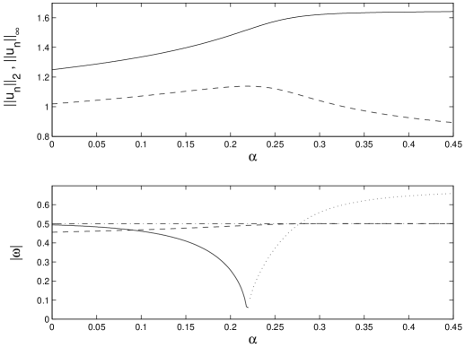
FIG. 4.: Top: the $L^{2}$ (solid line) and $L^{\infty}$ (dashed line) norms of the localized mode vs. $\alpha$. Bottom: the relevant point spectrum eigenvalues of the problem continued over $\alpha$. The solid line shows the pinning (or translational) mode that becomes unstable (dotted line) after $\alpha_{c}\approx 0.22$. The dashed line shows the breathing (or edge) mode, while the dash-dotted line indicates the band edge of the continuous spectrum.

Additional insight on the appearance of the instability is given in Fig. 4, where we examine the mode stability for different values of $\alpha$ (at $h=1$). The bottom panel of the figure shows the trajectory of the main eigenmodes of the point spectrum of the linearization around the solution. The solid line shows the translational or pinning (antisymmetric) mode, while the dashed line shows the edge or breathing (spatially symmetric) mode [32]. Notice that for $h=1$ (cf. Fig. 1 of Ref. [32]), the pinning mode has a larger frequency than the breathing mode. The band edge of the continuous spectrum which lies at $\Lambda=0.5$ [32] is shown by a dash-dotted line. As $\alpha$ is increased, it is clear that the breathing mode is “repelled” by the presence of the impurity towards the phonon band edge. On the contrary, the antisymmetric mode gradually approaches the origin and becomes unstable (dotted part of the relevant curve) for $\alpha>0.22$ (thereafter, for $\alpha>\alpha_{c}$ there appears an imaginary pair of eigenfrequencies). Perhaps it is even more interesting to examine the occurrence of this instability in the light of the top panels of the figure. The latter show the $L^{2}$ and $L^{\infty}$ norms of the solution as a function of $\alpha$. It is noteworthy that the occurrence of the instability coincides with the change of concavity of the $L^{2}$ norm, while it also coincides with a maximum of the $L^{\infty}$ norm. The above results suggest two additional numerical criteria that can be used to identify the appearance of the instability, namely

$$\frac{\partial^{2}||u||_{2}}{\partial\alpha^{2}}=0,$$ (12)

and

$$\frac{\partial||u||_{\infty}}{\partial\alpha}=0;\;\;\;\frac{\partial^{2}||u||_{\infty}}{\partial\alpha^{2}}<0.$$ (13)

IV Dynamical effects and asymmetric modes

To examine the dynamical development of the instability, once the solution becomes unstable for the supercritical values of $\alpha>\alpha_{c}$, we have performed direct numerical simulations of Eq. (1) with an initial condition consisting of an exact, unstable localized mode for $\alpha=0.3$, perturbed by small noise (of uniform distribution, and amplitude ranging from 0.0001 to 0.1). The scenario that is described was found to be generic for such perturbations of the unstable solution. It was thus found that as is shown in the top left panel of Fig. 5 for $t=200$, the unstable mode sustains a symmetry breaking, which cleaves it into another stable localized mode centered essentially at the neighboring (previous) lattice site ( see also the bottom right panel), and to a small-amplitude mobile pulse that propagates along the chain and carries an energy excess. It is worth noting that the original (unstable) eigenmode had 3 “main” sites oscillating at an amplitude of $\approx 0.9$, while the resulting breather is very strongly localized at a single site (of amplitude $\approx 1.7$).

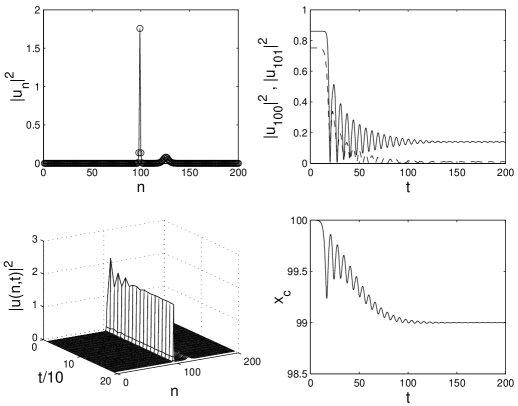
FIG. 5.: Development of the mode instability for $\alpha=0.3$ and $h=1$. The top left panel shows the mode spatial profile at $t=200$. The top right shows the modulus squared of the central site and of the site nearest to it, indicating relaxation to an exponentially localized configuration centered around the neighboring minimum (at $n\approx 99$). The bottom left panel shows a space time plot of the evolution of the modulus squared of the field, while the bottom right indicates the relaxation of the localized mode center from site $x_{c}\approx 100$ to the one with $x_{c}\approx 99$.

The trapping of the unstable mode by the neighboring site is consistent with the physical picture described by the effective Hamiltonian (6), when the mode overcomes the neighboring Peierls-Nabarro barrier and becomes localized by the next minimum. However, for smaller values of the lattice spacing $h$, when the Peierls-Nabarro barrier becomes negligible, the unstable localized mode can start its motion through the lattice under the action of the initial perturbation and as a result of the development of the symmetry-breaking instability. An example of the latter type is shown in Fig. 6 for the defect strength $\alpha=1$ and $h=0.5$.

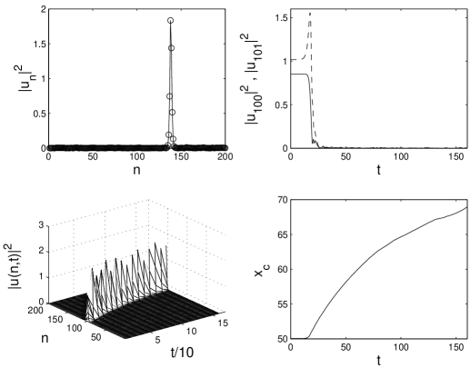
FIG. 6.: Same as in Fig. 5 but for $\alpha=1$ and $h=0.5$. Instability initiates the motion of a localized mode along the chain.

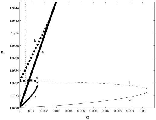
FIG. 7.: Bifurcation diagram of the asymmetric localized impurity modes. The thickest solid line (branch a) corresponds to the mode centered at $n_{0}=100$, while the corresponding dashed line (branch b), to the mode centered at $n_{0}=99.5$. The medium thickness solid line and the corresponding dashed one (branches c and d) are centered, for $\alpha=0$ at $n_{0}=99$ and $n_{0}=98.5$ respectively. The corresponding saddle-node bifurcation resulting at the disappearance of these branches occurs for $\alpha\approx 0.00147$. Finally, the thin solid and dashed lines (branches e and f) correspond to the cases of $n_{0}=98$ and $n_{0}=97.5$, respectively. The saddle-node bifurcation occurs here at $\alpha\approx 0.0105$. The dotted line at $\alpha=0.0005$ indicates the defect strength for which the mode profiles of the different branches are shown in Fig. 8. In the homogeneous case ($\alpha=0$) the array of minima and maxima of the Peierls barrier occurs for $x_{c}=m$ and $x_{c}=m+1/2$ ($m\in{\cal Z}$). Hence, the points with $x_{c}=100,99,98,97\dots$ have the same norm (the same is true for the branches with $x_{c}=99.5,98.5,97.5\dots$) for $\alpha=0$. In the presence of the impurity (e.g., for $\alpha\neq 0$), this shift invariance is broken. Thus we use the “original” (e.g., for $\alpha=0$) center position of the branch to classify them when $\alpha\neq 0$.

One of the most interesting findings of our study of the time evolution as a result of the mode instability is the effective “relaxation” of the unstable mode towards the mode centered at the neighboring (to the defect) site. The latter result prompted us to explore the modes in the vicinity of the defect. Due to symmetry, our study was restricted to modes on one side of the impurity site. The bifurcation diagram of the relevant branches of solutions is shown in Fig. 7 obtained for $h=0.5$. We have observed the relevant phenomenology to be generic, but report it for this value of the lattice spacing that necessitates narrower ranges of parameter sweeps (i.e., the same observations can be obtained for larger $h$, but due to the weaker coupling, they occur for considerably larger values of the defect strength $\alpha$).

The natural starting point for our analysis is the continuation from the case of an homogeneous lattice ($\alpha=0$), where the stationary modes are well-known to exist on a lattice site and between two consecutive lattice sites. Hence, in the homogeneous case we consider the branches centered at $n_{0}=100$ (branch a), $n_{0}=99.5$ (branch b), $n_{0}=99$ (c), $n_{0}=98.5$ (d), $n_{0}=97.5$ (e) and $n_{0}=97$ (f). We observe that at the instability point $a_{c}\approx 0.00252$, the stable branch a and the unstable branch b merge. The resulting branch is always unstable thereafter. For any other branch apart from the central one, we have found that the relevant stable (node) and unstable (saddle) solutions exist for a parameter interval that depends on the distance of the central site of the branch from the defect site; naturally, the branches whose central site is more remote from the defect are less affected by it (and exist for larger intervals of defect strengths). These branches eventually disappear in saddle-node bifurcations, as is observed for branches c and d and e and f in Fig. 7. A set of spatial profiles corresponding to the different branches are shown in Fig. 8 for the different branches of Fig. 7 and for $\alpha=0.0005$ (corresponding to the vertical dotted line in Fig. 7).

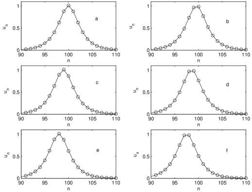
FIG. 8.: Spatial profiles of the localized modes corresponding to the branches (a) to (f) in Fig. 8 for the defect strength $\alpha=0.0005$. A repulsive impurity is located at the site $n_{0}=100$.

Disappearance of the relevant branches of static solutions is consonant with the mobility of the unstable modes for smaller values of $h$ observed in Fig. 6 above. For smaller values of $h$, the neighboring branches disappear for smaller defect strengths, hence allowing for no static solutions in the vicinity (in configuration space) of the unstable solution, thereby resulting in the mobility of the latter (i.e., the solution cannot be trapped in neighboring potential wells as these have disappeared). However, in the opposite case of large $h$, the lattice is strongly discrete and an adiabatic growth of the defect strength $\alpha$ leads to the mode motion from one stable state to its neighboring state (via an intermediate unstable mode) through a cascade of the bifurcation points.

V Conclusions

We have studied the existence and stability of nonlinear localized modes in the framework of the DNLS model. We have used a variational formalism to obtain the analytical result for the occurrence of an instability due to the interplay between attractive nonlinearity and repulsive impurity. We have examined the variational prediction by means of numerical bifurcation theory, linear stability analysis, as well as direct integration of the discrete lattice model. We have found the variational prediction (and its refinements) to be in reasonable agreement with the numerical results, attributing the discrepancies to the variation of the original profile with respect to the pre-selected ansatz. We have observed that the instability develops much before the solution becomes two-humped, and we have developed numerically motivated criteria for the identification of the instability. The study of the dynamical evolution of the unstable modes revealed the potential for mobile localized modes for smaller values of the lattice spacing, while it results in relaxation to the neighboring potential wells and the corresponding stable, static solutions. Finally, the bifurcation diagram has been explored as a function of the defect strength, using continuation from the homogeneous lattice case. We have found that for the branch corresponding to the defect site, the stable and nearest unstable solution branches merge at the instability point (producing a thereafter always unstable branch), while the neighboring sites corresponding stable and unstable branches disappear through collision via saddle-node bifurcations. Such a bifurcation scenario is in a perfect agreement with the concept of the Peierls potential that affects the mode motion in discrete systems.

PGK would like to thank J. Cuevas for stimulating discussions and for bringing to his attention the results of [18] prior to publication. He would also like to acknowledge partial support through a Faculty Research Grant of the University of Massachusetts and the Clay Foundation for support through a Special Project Prize Fellowship and the National Science Foundation for support through DMS-0204585. YSK acknowledges a support from the US Air Force-Far East Office and the Australian Research Council. ASK would like to acknowledge partial support from Royal Swedish Academy of Science.

REFERENCES

- [1] O.M. Braun and Yu.S. Kivshar, Phys. Rep. 306, 2 (1998); S. Flach and C.R. Willis, Phys. Rep. 295, 181 (1998). See also Physica 119D, (1999), a special volume edited by S. Flach and R.S. MacKay; D. Hennig, and G.P. Tsironis, Phys. Rep. 307, 334 (1999); P.G. Kevrekidis, K.Ø. Rasmussen, and A.R. Bishop, Int. J. Mod. Phys. B 15, 2833 (2001); A.J. Sievers and S. Takeno, Phys. Rev. Lett. 61, 970 (1988); S. Takeno and A.J. Sievers, Solid State Comm. 67, 1023 (1988).
- [2] A. Trombettoni and A. Smerzi, Phys. Rev. Lett. 86, 2353 (2001); J. Phys. B 34, 4711 (2001).
- [3] S.F. Mingaleev, Yu.S. Kivshar, and R.A. Sammut, Phys. Rev. E 62, 5777 (2000); S.F. Mingaleev and Yu.S. Kivshar, Phys. Rev. Lett. 86, 5474 (2001); D.N. Christodoulides and N.K. Efremidis, Opt. Lett. 27, 568 (2002).
- [4] D.N. Christodoulides and R.I. Joseph, Opt. Lett. 13, 794 (1988).
- [5] H.S. Eisenberg, Y. Silberberg, R. Morandotti, A.R. Boyd, and J.S. Aitchison, Phys. Rev. Lett. 81, 3383 (1998); R. Morandotti, H.S. Eisenberg, Y. Silberberg, M. Sorel, and J.S. Aitchison, Phys. Rev. Lett. 86, 3296 (2001).
- [6] A.A. Sukhorukov, Yu.S. Kivshar, H.S. Eisenberg, and Y. Silberberg, IEEE J. Quantum Electron. 39, January (2003).
- [7] D.N. Christodoulides and E.D. Eugenieva, Opt. Lett. 26, 1876 (2001); Phys. Rev. Lett. 87, 233901 (2001).
- [8] See e.g., A.A. Maradudin, Theoretical and Experimental Aspects of the Effects of Point Defects and Disorder on the Vibrations of Crystal (Academic Press, New York, 1966).
- [9] See e.g., I.M. Lifschitz, Nuovo Cimento, Suppl. 3, 716 (1956); I.M. Lifschitz and A.M. Kosevich, Rep. Progr. Phys. 29, 217 (1966).
- [10] A.F. Andreev, JETP Lett. 46, 584 (1987); A.V. Balatsky, Nature (London) 403 717 (2000).
- [11] M.I. Molina and G.P. Tsironis, Phys. Rev. B 47, 15330 (1993); G.P. Tsironis, M.I. Molina, and D. Hennig, Phys. Rev. E 50, 2365 (1994).
- [12] E. Lidorikis, K. Busch, Q. Li, C.T. Chan, and C.M. Soukoulis, Phys. Rev. B 56, 15090 (1997).
- [13] S.Y. Jin, E. Chow, V. Hietala, P.R. Villeneuve, and J.D. Joannopoulos, Science 282, 274 (1998); M.G. Khazhinsky and A.R. McGurn, Phys. Lett. A 237, 175 (1998).
- [14] M.M. Bogdan, A.S. Kovalev, and I.V. Gerasimchuk, Low Temp. Phys. 23, 145 (1997).
- [15] A.A. Sukhorukov, Yu.S. Kivshar, O. Bang, J.J. Rasmussen, and P.L. Christiansen, Phys. Rev. E 63, 036601 (2001).
- [16] K. Forinash, M. Peyrard, and B. Malomed, Phys. Rev. E 49, 3400 (1994).
- [17] W. Krolikowski and Yu.S. Kivshar, J. Opt. Soc. Am. B 13, 876 (1996).
- [18] J. Cuevas, F. Palmero, J.F.R. Archilla, and F.R. Romero (unpublished).
- [19] Yu.S. Kivshar, F. Zhang and A.S. Kovalev, Phys. Rev. B 55, 14265 (1997).
- [20] U. Peschel, R. Morandotti, J.S. Aitchison, H.S. Eisenberg, and Y. Silberberg, Appl. Phys. Lett., 75, 1348 (1999).
- [21] R. Morandotti, H.S. Eisenberg, D. Mandelik, Y. Silberberg, D. Modotto, M. Sorel, and J.S. Aitchison, “Interactions of discrete solitons with defects and interfaces”, in OSA Trends in Optics and Photonics (TOPS), Vol. 74, QELS’2002, OSA Technical Digest (OSA, Washington, DC, 2002), p. 239.
- [22] A.M. Kosevich and A.S. Kovalev, Sov. J. Low Temp. Phys. 1, 742 (1975).
- [23] A.S. Kovalev and M.M. Bogdan, Physics of Many-particle Systems 13, 20 (1988) (in Russian).
- [24] V.L. Indenbom, Sov. Phys. Crystallogr. 3, 193 (1959).
- [25] S.F. Mingaleev and Yu.S. Kivshar, J. Opt. Soc. Am. B 19, 2241 (2002).
- [26] I.V. Gerasimchuk and A.S. Kovalev, Low Temp. Phys. 26, 586 (2000).
- [27] A.A. Sukhorukov and Yu.S. Kivshar, Phys. Rev. Lett. 87, 083901 (2001); Phys. Rev. E 65, 036609 (2002).
- [28] See e.g., P.M. Morse and H. Feshbach, Methods of Theoretical Physics (McGraw-Hill, New York, 1953), p. 466.
- [29] T. Kapitula, P.G. Kevrekidis, and B.A. Malomed, Phys. Rev. E 63, 036604 (2001).
- [30] T. Kapitula, Physica D 156, 186 (2001).
- [31] D.E. Pelinovsky and Yu.S. Kivshar, Phys. Rev. E 62, 8668 (2000).
- [32] M. Johansson and S. Aubry, Phys. Rev. E 61, 5864 (2000).