Quantization of Classical Maps with tunable Ruelle-Pollicott Resonances

Abstract

We investigate the correspondence between the decay of correlation in classical systems, governed by Ruelle–Pollicott resonances, and the properties of the corresponding quantum systems. For this purpose we construct classical dynamics with controllable resonances together with their quantum counterparts. As an application of such tailormade resonances we reveal the role of Ruelle–Pollicott resonances for the localization properties of quantum energy eigenstates.

I Introduction

The quantum-classical correspondence of non-integrable systems has been studied for a long time. In recent years the role of classical Ruelle–Pollicott resonances for the dynamics of the quantum counterparts has become a point of interest Altshuler ; Zirnbauer ; Pance ; chris1 . The classical time evolution can be described in the Liouville picture as the propagation of the phase-space density $\rho(x,t)$, where $x$ denotes a point in phase space. The corresponding propagator $P$ is called Frobenius–Perron (FP) operator and can be defined by

$$\rho(x,t)=\int{\rm d}x^{\prime}\,\delta(x-F^{t}(x^{\prime}))\rho(x^{\prime},0)\equiv P^{t}\rho(x,0)\ ,$$ (1)

where $F$ is the flow in the phase space generated by the dynamics $x(t)=F^{t}(x(0))$. The poles of the resolvent of this operator are the Ruelle–Pollicott resonances Ruelle ; Pollicott . It turns out that these resonances correspond to decay rates of classical correlation functions describing the relaxation process in a chaotic system GaspardBook . The presence of the Ruelle–Pollicott resonances related to slow decay of correlations can explain non-universal behaviour of the corresponding quantum system, i.e. deviations from predictions of the random-matrix theory (RMT) analyzed e.g. in HaakeBook .

In order to reveal such effects of resonances we first construct a classical system with an isolated, controllable resonance which can be computed analytically. We focus our considerations on dynamical systems with compact phase spaces, in particular the unit sphere. Periodic driving destroys integrability, where the stroboscopic description of such a dynamics is given by a Hamiltonian map. For this case the Ruelle–Pollicott resonances are located inside the unit circle of the complex plane, while decay rates are related to the moduli of resonances. For the quantum counterpart the stroboscopic description of the propagation of wave functions is given by a unitary Floquet operator. The eigenphases of that operator are also called quasi-eigenenergies.

Analytical calculations of Ruelle-Pollicott resonances are feasible for purely hyperbolic systems ChaosBook ; Nonnenm . We introduce dynamics which are not Hamiltonian (continuous) but still area preserving, coupled baker maps on the sphere. These model systems are introduced in Sec. II, where we also show how to find their periodic orbits, approximate resonances and calculate the traces of the Frobenius–Perron operators associated with them. Construction of the corresponding quantum propagators together with the comparison of quantum and classical dynamics is presented in Sec. III. In Sec. IV we investigate how Ruelle–Pollicott resonances give rise to the deviations from the random–matrix theory. Eventually in Sec. V we present the model of coupled random matrices which can be considered as a simplification of the systems introduced in Sec. II.

II Coupled baker maps

We are interested in classical dynamical systems for which there exists a Ruelle–Pollicott resonance with large modulus. Such a resonance governs the long-time behaviour of the system and is easy to detect.

The idea standing behind our model systems is rather simple. Suppose our system is initially composed out of two disconnected subsystems. An arbitrary initial density placed in one of those subsystems will not spread into the other subsystem. The system as a whole will thus have two invariant (stationary) densities, one for each subsystem (and the linear combinations thereof). This fact will be reflected in the spectrum of the Frobenius–Perron operator as a doubly degenerated eigenvalue $\lambda_{1}=\lambda_{2}=1$. However, if we introduce a small coupling between both subsystems, the density from one subsystem will slowly leak into the other one and eventually reach the invariant density of the entire system. As a result of the coupling the degeneracy of the spectrum will be lifted. The largest eigenvalue $\lambda_{1}=1$ corresponds to the unique invariant density of the entire system, while the other eigenvalue $\lambda_{2}$ with $|\lambda_{2}|=1-\epsilon<1$ corresponds to a metastable state. The smaller the spectral gap $\epsilon$, the longer the decay time of the state.

For the internal dynamics of both subsystems we choose the standard baker map acting on a unit square — a well known model of chaotic dynamics Arnold . One possible way to introduce the coupling is described by

$$(y^{\prime},x^{\prime})=F(y,x)=\left\{\begin{array}[]{ll}(2y-1,x/2+1/2)&y\geq z,x\leq 1/2\\ (2y-1,x/2+1/4)&y\in[1/2,z),x\leq 1/2\\ (2y,x/2)&y<1/2,x\leq 1/2\\ (2y-1,x/2)&y\geq z,x>1/2\\ (2y-1,x/2+1/4)&y\in[1/2,z),x>1/2\\ (2y,x/2+1/2)&y<1/2,x>1/2\\ \end{array}\right.\ ,$$ (2)

whose action is depicted in Fig. 1.

Figure 1: Map on the unit square defined by (2) for $z=3/4$.

In the limiting case $z=1$ the parts $A_{1}$ and $A_{2}$ vanish and there exist two separated subsystems, with indices 1 and 2 (each of them equivalent to the standard baker map). For $z<1$ both subsystems are coupled together. To describe the strength of the coupling we introduce a parameter $\Delta=1-z$ which varies from $0$ to $1/2$.

II.1 The system with a negative coupling

We now present a slightly modified version of the map (2) which results in the resonance of a large modulus with negative sign. Thus we call both versions of the model as “positive” and “negative” coupling depending on the sign of the resonance.

We start again with two uncoupled baker maps. In addition to their internal dynamics, we assume that in every iteration of the map both subsystems exchange their positions. The FP operator corresponding to such a system will thus have two eigenvalues of unit modulus: $\lambda_{1}=+1$ and $\lambda_{2}=-1$. Any small coupling of both subsystems will cause the density placed in one subsystem to slowly leak into the other one so the entire system will possess a resonance of large modulus and its negative sign will reflect oscillatory nature of the system.

The version of the coupling that we have chosen is presented in Fig. 2 and is defined by

$$(y^{\prime},x^{\prime})=F(y,x)=\left\{\begin{array}[]{ll}(2y-1,x/2+1/2)&y\geq 1/2,x\leq 1/2\\ (2y,x/2+3/4)&y\in[z,1/2),x\leq 1/2\\ (2y,x/2)&y<z,x\leq 1/2\\ (2y-1,x/2)&y\geq 1/2,x>1/2\\ (2y,x/2-1/4)&y\in[z,1/2),x>1/2\\ (2y,x/2+1/2)&y<z,x>1/2\\ \end{array}\right.\ .$$ (3)

Figure 2: Action of the map (3) for $z=1/4$.

Accordingly for this system the coupling strength parameter is given by $\Delta=z$. The full coupling ($\Delta=1/2$) limits of systems (2) and (3) coincide and correspond to the baker map on the sphere defined in Pakonski1999 .

Our ultimate goal is to construct a quantum system corresponding to the classical system with a large resonance and to investigate the influence of the classical resonance on the properties of the quantum system. For this purpose we make use of periodic orbits of the classical system and the spectrum of the Frobenius–Perron operator corresponding to the classical system — which we will approximate by introduction of a stochastic perturbation into the system. Hence the following two sections are devoted to these subjects.

II.2 Periodic orbits of the classical system

For the determination of the periodic orbits of the system we will use the Markov partition. For any dynamical system $F$ it is defined as a such partition $\mathcal{C}$ of the phase space into $K$ cells that the borders of each cell are composed of segments of stable and unstable manifolds of the system. Additionally this partition has to fulfill

$$F(\partial_{s}\mathcal{C}) \subset \partial_{s}\mathcal{C},$$ (4)

$$F^{-1}(\partial_{u}\mathcal{C}) \subset \partial_{u}\mathcal{C},$$ (5)

so the image of the stable part of the partition boundary $\partial_{s}\mathcal{C}$ is contained in $\partial_{s}\mathcal{C}$ and the unstable part of the boundary $\partial_{u}\mathcal{C}$ contains its preimage GaspardBook . Such a partition generates a symbolic dynamics with a $K$-letter alphabet which is a topological Markov chain. In the following we will concentrate on the system (2), since most of the results below can be translated directly to system (3), and we will only emphasize important differences.

For system (2) we are able to find a Markov partition for several values of the coupling parameter $\Delta$. For example, for $\Delta=1/2^{k}$ with natural $k$ this partition is defined by a set of horizontal lines $y_{i}=1-1/2^{i}$ where $i=1,\ldots,k$ and a vertical line at $x=1/2$. It is easy to verify that under the action of (2) each coordinate $y_{i}$ is mapped to $y_{i-1}$ and eventually tends to $y_{1}=1/2$ which is mapped to $y=0$.

Basing on this partition we can construct a transition matrix $\mathbf{T}$ with entries $T_{ij}$ equal to probabilities that the system passes from the cell $i$ to the cell $j$. For simple piecewise linear maps an agreement between the resonance of the corresponding Frobenius–Perron operator with the second largest modulus and the eigenvalue of this matrix was observed ChaosBook . The dimension of the transition matrix for the system (2) with $\Delta=1/2^{k}$ grows linearly with $k$ according to $K=\dim\mathbf{T}=2(k+1)$, and one can easily obtain its eigenvalues. For instance, for $k=3$ ($\Delta=1/8$) the second largest eigenvalue is equal $\lambda_{2}^{+}\approx-0.8846$, while in case of negative coupling (3) $\lambda_{2}^{-}=-\lambda_{2}^{+}$ — see Appendix A.

The transition matrix $\mathbf{T}$ for the system (2) enables us to specify periodic orbits of the system. The number of periodic points is given directly by

$$|\{(x,y):(x,y)=F^{n}(x,y)\}|=\mathop{\operator@font tr}\mathsf{T}^{n}\ ,$$ (6)

where we introduced the connectivity matrix $\mathsf{T}$ (sometimes called topological transition matrix GaspardBook ) defined as a transition matrix with all non-zero entries replaced by 1,

$$\mathsf{T}_{ij}=\left\{\begin{array}[]{ll}1&\mathrm{if}\ \mathbf{T}_{ij}>0\\ 0&\mathrm{otherwise}\end{array}\right.\ .$$ (7)

It is worth to note that formula (6) is valid only if none of the periodic orbit crosses the boundary of the partition — otherwise we have to take into account that a given symbolic sequence may not define a point in the phase space uniquely, so it might happen that one orbit is counted more than once. One can verify that there is no such problem for system (2), but this is not the case for system (3). Periodic sequences $\omega_{1}=B_{1}A_{2}$ and $\omega_{2}=B_{2}A_{1}$ (see Fig. 2) correspond to the orbits starting from the same initial point $x=1/2$, $y=1/3$ which belongs to the partition line. This fact needs to be taken into account during calculations of the traces of the FP operator.

Note also that the systems (2) and (3), originally defined on the square (torus) may also represent dynamics on the sphere, where $y\rightarrow\cos\theta$ and $x\rightarrow\varphi$. In this case the entire line $y=0$ has to be identified with the south pole (and line $y=1$ with the north pole, respectively), so the number of periodic orbits in both systems may differ.

II.3 Approximation of the Frobenius–Perron spectrum

We are not able to find analytically resonances of the systems (2) and (3) (apart from the second largest which we obtain from the transition matrix). To approximate them we follow an approach developed in OPSZ2000 ; fishman ; weber1 ; OZ2001 ; weber2 and introduce a stochastic perturbation into the system. This allows us to represent the Frobenius–Perron operator corresponding to the system with noise as a finite dimensional matrix.

In Section III we define quantum propagators corresponding to systems (2) and (3). In order to use well known SU(2) coherent states Radcliffe ; Arecchi ; Glauber ; Perelomov we convert appropriate definitions of the classical systems into the unit sphere by applying the Mercator projection. More formally, we replace $x$ with $\varphi=2\pi x$ and $y$ with $t=\cos\theta=2y-1$, where $\varphi$ and $\theta$ are the usual spherical coordinates. The parameter $\Delta\in(0,\frac{1}{2})$ defined previously plays the same role of the coupling constant. Accordingly we should approximate resonances for the classical system defined on the sphere. A possible choice of the probability density of the stochastic perturbation which transforms a point $\Omega=(\theta,\varphi)$ on the sphere into $\Omega^{\prime}=(\theta^{\prime},\varphi^{\prime})$ is

$$\mathcal{P}_{M}(\Omega^{\prime},\Omega)=$$

$$= \frac{M+1}{4\pi}\left(\frac{1+\cos\Xi}{2}\right)^{M}$$

$$= \frac{M+1}{4\pi}\sum_{k,l=0}^{M}{M\choose k}{M\choose l}(\sin^{k+l}\frac{\theta}{2}\cos^{2M-(k+l)}\frac{\theta}{2}{\rm e}^{{\rm i}(l-k)\varphi})\times$$

$$\times(\sin^{k+l}\frac{\theta^{\prime}}{2}\cos^{2M-(k+l)}\frac{\theta^{\prime}}{2}{\rm e}^{-{\rm i}(l-k)\varphi^{\prime}})\ ,$$

where $M$ is an arbitrary natural number. Here $\Xi$ is the angle formed by two vectors pointing toward the points $\Omega$ and $\Omega^{\prime}$ on the sphere. As discussed in OPSZ2000 ; OZ2001 the matrix representation of the Frobenius–Perron operator for system with such a noise is finite dimensional — the last equation in (II.3) helps to identify the basis functions of the matrix representation. For the probability distribution (II.3) the dimension of the matrix is $(M+1)^{2}$ and grows to infinity in the deterministic limit $M\rightarrow\infty$, for which $\mathcal{P}_{\infty}(\Omega^{\prime},\Omega)=\delta(\Omega-\Omega^{\prime})$ with respect to the uniform measure on the sphere, ${\rm d}\Omega=\sin\theta{\rm d}\theta\,{\rm d}\varphi$. However, for any finite $M$ one obtains a finite representation of the FP operator and may diagonalize it numerically. In this way we obtain the exact spectrum for the system with noise and by decreasing the noise amplitude we can approximate the resonances of the deterministic system. Fig. 3 presents the dependence of the modulus of the second largest eigenvalue $\lambda_{2}$ of systems (2) and (3) subjected to additive noise (II.3) on the noise parameter $M$. The deterministic limit — represented in Fig. 3 as a dashed line — is the same for both systems and is obtained from the transition matrix defined in the previous section.

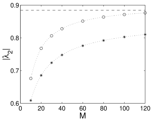
Figure 3: Dependence of the modulus of the second largest eigenvalue of the FP operator for the stochastically perturbed coupled baker maps on the sphere on the noise parameter $M$. Values for the system (2) and (3) are represented by $\circ$ and $\ast$, respectively (in both cases $\Delta=1/8$). The dashed line represents the deterministic limit.

The most striking observation is that although the deterministic value of $|\lambda_{2}|$ for both systems is the same, the approximations of $\lambda_{2}$ for a given value of the noise parameter $M$ differ. This can be understood with the help of Fig. 4, where we showed the result of the second iteration of the corresponding systems.

Figure 4: Second iteration of the systems (2) (left) and (3) (right).

The total length of the boundary between subsystem $1$ and $2$ for the negative coupling (right plot) is one and half times larger than for the positive coupling. Thus in the case of the negative coupling it is more likely that points will move from one subsystem to the other one under the action of the stochastic perturbation. The overall decay rate in the presence of the noise is thus faster than in the case of the positive coupling which is reflected in the spectrum as a smaller modulus of the subleading eigenvalue $\lambda_{2}$.

II.4 Traces of the Frobenius–Perron operator

For the semiclassical analysis we will need the traces of the Frobenius–Perron operator $P$ associated with the classical system. Approximation of the traces with the help of stochastic perturbation is straightforward, since we obtain eigenvalues $\lambda_{i}$ of the FP operator for the noisy system and we can calculate the traces directly from the definition

$$\mathop{\operator@font tr}P^{n}=\sum_{i}\lambda_{i}^{n}\ .$$ (9)

In order to calculate the traces with the use of periodic orbits we will use the integral representation of the FP operator (1). To obtain the expression for the traces it is sufficient to identify initial and final points in this expression, that is

$$\mathop{\operator@font tr}P^{n}=\int{\rm d}\Omega\,\delta(\Omega-F^{n}(\Omega))=\sum_{\Omega_{i}:\Omega_{i}=F^{n}(\Omega_{i})}\frac{1}{|\det(1-J^{n}(\Omega_{i}))|}\ ,$$ (10)

where $J^{n}(\Omega_{i})$ denotes the Jacobian matrix of the mapping $F^{n}$ evaluated in point $\Omega_{i}$ and we make use of the properties of the $\delta$ function in the last equality. The calculation of the denominator in (10) is easy, since our systems are purely hyperbolic with constant stretching and squeezing by a factor of two. Thus the contribution of each fixpoint to the trace of $P^{n}$ is equal to $[2^{n}+2^{-n}-2]^{-1}$. The only periodic points which need special attention are the south and the north pole since — due to the discontinuities — expression (10) is not well defined in these points. In order to calculate the contribution from these points we “regularized” the integral (10) — see Appendix B.

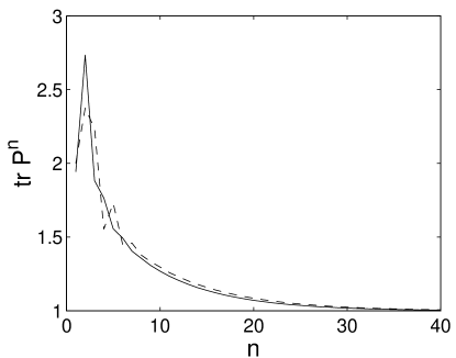
Figure 5: Traces of the FP operator: (a) positive coupling (2) with $\Delta=1/8$, (b) negative coupling (3) ($\Delta=1/8$) and (c) full coupling corresponding to the system (2) with $\Delta=1/2$ (or to (3) also with $\Delta=1/2$). Solid lines represent traces calculated from the approximate spectrum of the FP operator while the traces obtained from the periodic orbits are plotted with dashed lines.

Having done that we can combine the contribution of the periodic points with their numbers calculated from (6). The traces, Fig. 5, calculated from the approximate spectrum and periodic orbits are represented by solid and dashed lines, respectively. These numerical results demonstrate good agreement between two different methods of computing the traces of the FP operator. Discrepancies visible in Fig. 5b and 5c are due to the fact that for the system (3) the effective coupling is stronger as discussed at the end of Sec. II.3.

III Quantum propagator

In the construction of the quantum propagator corresponding to the systems (2) and (3) we rely on the results presented in Pakonski1999 in which the quantum baker map was defined on the sphere. The corresponding classical system is obtained from (2) and (3) in the full coupling limit $\Delta=1/2$ and its action is visualized in Fig. 6.

Figure 6: Baker map on the sphere in Mercator projection $(t=\cos\theta,\varphi)$. This map is the full coupling limit ($\Delta=1/2$) of the systems (2) and (3).

The construction of the quantum system is based on the matrix representation of the rotation around the $y$–axis by an angle of $\pi/2$

$$R_{m^{\prime},m}=\langle j,m|{\rm e}^{-{\rm i}\frac{\pi}{2}\hat{J}_{y}}|j,m^{\prime}\rangle\ ,$$ (11)

where $\hat{J}_{i}$ is the $i$-th component of the angular momentum operator $\hat{J}$ and $|j,m\rangle$ is an eigenvector of the $\hat{J}_{z}$ operator, $\hat{J}_{z}|j,m\rangle=m|j,m\rangle$ with $m=-j,\ldots,j$. In the following we choose half–integer spin values $j$, so the size of the rotation matrix $N=2j+1$ is even. The resulting quantum propagator is defined as Pakonski1999

$$\hat{U}_{B}=R^{-1}\left[\begin{array}[]{cc}R^{\prime}&0\\ 0&R^{\prime\prime}\end{array}\right]\ ,$$ (12)

where $R^{\prime}$ and $R^{\prime\prime}$ are matrices created by taking halves (respectively upper and lower) of every second column of the rescaled Wigner rotation matrix $R$

$$R^{\prime}_{k,m} = \sqrt{2}\,R_{k,2m-j}\qquad k,m=\frac{1}{2},\ldots,j\ ,$$ (13)

$$R^{\prime\prime}_{k,m} = \sqrt{2}\,R_{k,2m+j}\qquad k,m=-j,\ldots,-\frac{1}{2}\ .$$ (14)

The construction (12) is similar to the original quantum map on the torus proposed by Balazs and Voros BV : instead of the Fourier matrix we use the Wigner rotation matrix $R$.

Now it is crucial to note that if we additionally exchange the parts $A_{1}^{\prime}$ and $A_{2}^{\prime}$ in Fig. (6), we obtain the uncoupled version of the map (2) for $\Delta=0$. The same happens if we exchange the parts $C_{1}^{\prime}$ and $C_{2}^{\prime}$ — we obtain then map (3) for $\Delta=0$. On the other hand a partial exchange of these regions will result in maps with $\Delta>0$.

The only question left is how to modify the definition of the quantum propagator in order to obtain the above mentioned exchange. It is sufficient to swap the cell $A_{1}$ with $A_{2}$ in Fig. 6 (or $C_{1}$ with $C_{2}$), or their parts, before applying the operator $\hat{U}_{B}$ from (12). Such an exchange may be accomplished by a rotation of the part of northern or southern hemisphere (for map (2) and (3), respectively) around the $z$–axis by angle $\pi$. This procedure is presented in Fig. 7 where this partial rotation is denoted by $R_{N}(\Delta)$ and $R_{S}(\Delta)$.

Figure 7: Construction of the maps (2) (a) and (3) (b) with use of the baker map on the sphere $F_{B}$ (cf. Fig. 6). Exchange of the cells $B_{1}\leftrightarrow B_{2}$ is denoted by $R_{N}(\Delta)$ and $R_{S}(\Delta)$ respectively.

Quantum operators corresponding to these rotations have simple representation in the $|j,m\rangle$ basis, since they are just multiplication of the vector of coefficients by a phase factor ${\rm e}^{-{\rm i}m\pi}$. In both cases the matrix representation is diagonal and for the “positive” coupling (2) the diagonal elements are equal

$$\hat{R}_{N}(\Delta)_{k,k}=\left\{\begin{array}[]{lll}1&\mathrm{for}&k<N\Delta\\ {\rm e}^{-{\rm i}(j-k+1)\pi}&\mathrm{for}&k\in(N\Delta,N/2)\\ 1&\mathrm{for}&k>N/2\end{array}\right.\ ,$$ (15)

while for “negative” coupling (3) the appropriate rotation operator has the following representation

$$\hat{R}_{S}(\Delta)_{k,k}=\left\{\begin{array}[]{lll}1&\mathrm{for}&k<N/2\\ {\rm e}^{-{\rm i}(j-k+1)\pi}&\mathrm{for}&k\in(N/2,N(1-\Delta))\\ 1&\mathrm{for}&k>N(1-\Delta)\end{array}\right.\ ,$$ (16)

where $N=2j+1$ is the dimension of the Hilbert space (we confine ourself to such values of $N$ and $\Delta$ that $N\Delta$ is integer). Using these operators we define unitary quantum maps corresponding to classical systems (2) and (3), respectively,

$$\hat{U}_{N} = \hat{U}_{B}\hat{R}_{N}(\Delta)$$ (17)

$$\hat{U}_{S} = \hat{U}_{B}\hat{R}_{S}(\Delta)\ ,$$ (18)

with $\hat{U}_{B}$ defined by Eq. (12).

III.1 Comparison of classical and quantum dynamics

In order to illustrate correctness of the proposed construction of the quantum propagators, we make use of periodic orbits of the classical systems. Suppose that for initial conditions for quantum dynamics we choose a wave function localized around some periodic point of the classical system. After the time equal to the period of the classical orbit the probability of measuring the system near the initial point in the phase space should be large. More precisely, for the initial state we choose the SU(2) coherent state $|\theta,\varphi\rangle$ localized in point $(\theta,\varphi)$. In the angular momentum representation a coherent state can be generated by a rotation of the state $|j,m=j\rangle$, which fulfills the smallest uncertainty relation Arecchi ; Glauber , as $|\theta,\varphi\rangle=R(\theta,\varphi)|j,j\rangle$. Now we will investigate the so called return probability

$$|Q_{U^{n}}(\theta,\varphi)|^{2}=|\langle\theta,\varphi|U^{n}|\theta,\varphi\rangle|^{2}\ ,$$ (19)

where $U$ is the quantum propagator. The $Q$ function of an operator $A$ is defined as

$$Q_{A}=\langle\theta,\varphi|A|\theta,\varphi\rangle\ .$$ (20)

For density operators the $Q$ function is also called Husimi function.

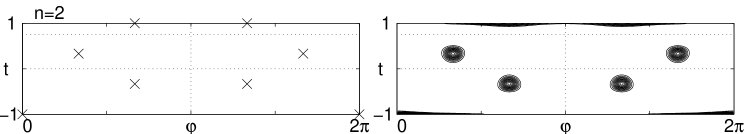
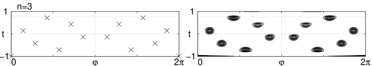
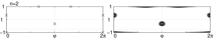
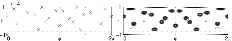
Figure 8: Classical periodic orbits (left hand side) for the systems (17) (upper part) and (18) (lower part) versus quantum return probability (19) for selected lengths $n$ of the orbits ($\Delta=1/8$).

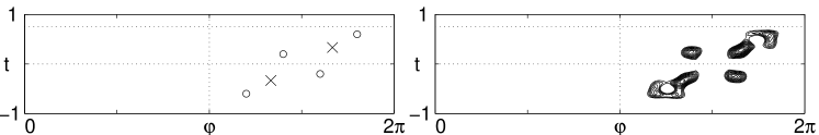
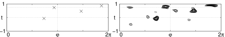
Figure 9: Periodic orbits of the classical system (left hand side) together with Husimi functions $Q_{|\psi\rangle\langle\psi|}$ of selected eigenvectors of quantum propagators showing corresponding scars. Upper part regards the model with positive coupling and shows that the selected eigenvector is scared by two orbits — period–2 orbit denoted on left hand side by $\times$ and period 4 orbit denoted by $\circ$. Lower part is for the system with negative coupling and in this case the selected eigenvector is scarred along period–4 orbit of the classical system. In both cases $\Delta=1/8$.

In a vicinity of the points $(\theta,\varphi)$, corresponding to periodic points of orbits of length $n$, we may expect large values of the return probability. The functions $|Q_{U^{n}}(\theta,\varphi)|^{2}$ for systems (17) and (18) are presented in Fig. 8: observe an agreement between maxima of the quantum return probability (19) and the periodic points of the classical system.

To emphasize the fact that regular periodic points, that is those indicated by corresponding symbolic dynamics, have much more influence than periodic points resulting from the boundary conditions we only showed points obtained from the Markov partition — without corrections resulting from the topology of the system. For example the line $t=1$ is one point (north pole) so a periodic orbit of length two for this value of $t$ coordinate is a fixpoint of the map. However, one can see that quantum return probability for this point is much higher for even iterations than for the odd ones.

One can also notice that some eigenvectors of the quantum propagator are scarred Heller ; Heller1 ; Heller2 ; Kus ; Stockmann by classical periodic orbits which is shown in Fig. 9. We conclude thus, that the procedure presented above indeed gives as a result quantum systems which correspond to (2) and (3).

IV Averaged Overlaps of Husimi Eigenfunctions

We here discuss how Ruelle–Pollicott resonances rise deviations from random-matrix theory as an application of tailormade resonances. In chris it has been shown that the classical resonances lead to semiclassical corrections of the localization of quantum eigenstates. In particular, it was shown that the probability of finding strongly phase-space overlapping quantum eigenfunctions increases if the difference of their (quasi-)eigenenergies is close to the phase of a classical resonance which corresponds to a slow correlation decay. On the other hand, if a pair of eigenfunctions strongly overlaps then each of them must be localized (scarred) in the same phase-space regions.

In contrast to the numerical results of chris which were obtained from a system with a classical mixed phase space we have here completely analytical classical results. Indeed, we do not calculate the resonances analytically, but for our purpose the traces of the Frobenius–Perron operator are sufficient. Here we briefly review those results that are relevant for the present discussion.

We focus our investigation on pure-state Husimi functions of projectors of Floquet eigenstates, i.e. the phase-space representation of (quasi-)energy eigenstates,

$$Q_{kk}\equiv Q_{|\phi_{k}\rangle\langle\phi_{k}|}=|\langle\theta,\varphi|\phi_{k}\rangle|^{2}\,.$$ (21)

Due to the normalization of a density operator, $\mathop{\operator@font tr}\rho=1$, the Husimi functions are $L^{1}$ normalized as

$$\frac{N}{4\pi}\int{\rm d}\Omega\,Q_{\rho}(\theta,\varphi)=1\,.$$ (22)

As a measure for phase-space localization we introduce the $L^{2}$ norm of a Husimi function,

$$||Q_{kk}||^{2}=\int{\rm d}\Omega\,|\langle\theta,\varphi|\phi_{k}\rangle|^{4}\,,$$ (23)

which is the inverse participation ratio with respect to coherent states. Another property of interest is the phase-space overlap of two Husimi functions,

$$||Q_{ik}||^{2}=\int{\rm d}\Omega\,|\langle\theta,\varphi|\phi_{i}\rangle|^{2}|\langle\theta,\varphi|\phi_{k}\rangle|^{2}\,.$$ (24)

The notation $Q_{ik}$ is used, since the phase-space overlap is the same as the $L^{2}$ norm of the “skew” Husimi function $Q_{|\phi_{i}\rangle\langle\phi_{k}|}$. The physical meaning of the overlaps becomes obvious from Schwarz’ inequality,

$$||Q_{ik}||^{2}\leq||Q_{ii}||\,||Q_{kk}||\,.$$ (25)

For large values of $||Q_{ik}||^{2}$ both Husimi functions must be localized in the same phase-space regions.

The introduced measures, $L^{2}$ norm or phase-space overlap, prove amenable to semiclassical considerations. It might be obvious that the return probability becomes

$$\frac{N}{4\pi}|\langle\theta,\varphi|U^{n}|\theta,\varphi\rangle|^{2}\mbox{$\,{}_{{}_{N\rightarrow\infty}}\!\!\!\!\!\!\!\!\!\!\!\longrightarrow\,$}\delta(\Omega-F^{n}(\Omega))$$ (26)

in the classical limit. Integration over phase space leads to the trace of the Frobenius-Perron operator,

$$\frac{N}{4\pi}\int{\rm d}\Omega\,|\langle\theta,\varphi|U^{n}|\theta,\varphi\rangle|^{2}\mbox{$\,{}_{{}_{N\rightarrow\infty}}\!\!\!\!\!\!\!\!\!\!\!\longrightarrow\,$}\mathop{\operator@font tr}P^{n}\,.$$ (27)

Introducing the Floquet eigenstates on the left hand side one finds

$$\frac{N}{4\pi}\int{\rm d}\Omega\,|\langle\theta,\varphi|U^{n}|\theta,\varphi\rangle|^{2} = \frac{N}{4\pi}\int{\rm d}\Omega\,\left|\sum_{k}|\langle\theta,\varphi|\phi_{k}\rangle|^{2}{\rm e}^{-{\rm i}n\phi_{k}}\right|^{2}$$ (28)

$$= \frac{N}{4\pi}\sum\limits_{ik}||Q_{ik}||^{2}\,{\rm e}^{-{\rm i}n(\phi_{i}-\phi_{k})}\,.$$

Fourier transformation of the latter expression leads to a sum of $\delta$ functions weighted by $L^{2}$ norms,

$$\sum\limits_{n=-\infty}^{\infty}\frac{{\rm e}^{{\rm i}n\omega}}{2\pi}\sum\limits_{ik}||Q_{ik}||^{2}\,{\rm e}^{-{\rm i}n(\phi_{i}-\phi_{k})}=\sum\limits_{ik}||Q_{ik}||^{2}\,\delta(\omega-(\phi_{i}-\phi_{k}))\,.$$ (29)

For finite Hilbert-space dimension $N$ the relation (27) might be valid for finite times $|n|\leq{\cal N}$. The truncated Fourier transform leads to a sum of smoothed $\delta$ functions,

$$\overline{||Q_{ik}||^{2}}^{\Delta\omega}(\omega)=\frac{4\pi}{N}\sum_{n=-{\cal N}}^{\cal N}\mathop{\operator@font tr}P^{n}\frac{{\rm e}^{{\rm i}n\omega}}{2\pi}\,.$$ (30)

The stationary eigenvalue $1$ will be dropped; it would lead to a $\delta$ function after Fourier transformation in the limit ${\cal N}\rightarrow\infty$. To this end we identify the stationary eigenvalue in the Husimi representation. In chris it has been shown that the stationary eigenvalue is related to the $L^{1}$ norms of Husimi functions. It turns out that the eigenvalue 1 can be dropped on the right hand side of (30) if one replaces the Husimi functions $Q_{kk}$ by $Q_{kk}^{\prime}=Q_{kk}-\frac{1}{N}$ on the left hand side, where $\int{\rm d}\Omega\,Q_{kk}^{\prime}=0$. (The prime will be dropped in the following.) For $n=0$ the integral on the left hand side of (27) gives the dimension $N$. We replace the traces by sums of the Ruelle-Pollicott resonances (9) and make use of the symmetry $\mathop{\operator@font tr}P^{-n}=\mathop{\operator@font tr}P^{n}$,

$$\overline{||Q_{ik}||^{2}}^{\Delta\omega}(\omega)=2\frac{N-1}{N}+\frac{4}{N}\sum_{n=1}^{\cal N}\sum_{\nu}\lambda^{n}_{\nu}\cos n\omega\,.$$ (31)

Note that the eigenvalue $1$ is also dropped in the leading order term. Assuming that the density of differences of Floquet eigenphases is almost constant, $N^{2}/2\pi$, we finally get the result that the overlaps averaged over an interval $\Delta\omega$ of differences of Floquet eigenphases ($\omega_{ik}=\phi_{i}-\phi_{k}$) are given by traces of the Frobenius–Perron operator, i.e. Ruelle–Pollicott resonances,

$$\left\langle||Q_{ik}||^{2}\right\rangle(\omega) = \frac{4\pi}{N^{2}}\left(1-\frac{1}{N}+\frac{2}{N}\sum_{n=1}^{\infty}({\rm tr}P^{n}-1)\cos n\omega\right)$$ (32)

$$= \frac{4\pi}{N^{2}}\left(1-\frac{1}{N}+\frac{2}{N}\sum_{\nu}\sum_{n=1}^{\infty}\lambda_{\nu}^{n}\cos n\omega\right)\,.$$

The constant term in parenthesis coincides up to the order $N^{-2}$ with the result of RMT chris , $\left\langle||Q_{ik}||^{2}\right\rangle_{\rm RMT}=\frac{4\pi}{N(N+1)}$. The traces of the Frobenius–Perron operator are expanded in sums of the Ruelle–Pollicott resonances, where a Fourier transform of each resonance leads to a periodic Lorentzian distribution displaced by the phase of the resonance. Note that the resonances are real or appear as complex conjugated pairs.

The averaged phase-space overlaps (32) might be understood as a scar correlation function. Due to the Schwarz’ inequality (25) the probability to find a pair of scarred eigenfunctions becomes large if the difference of their eigenenergies is close to the phase of a resonance of large modulus, i.e. close to the position of a strongly peaked Lorentzian.

For numerical results we first have smoothed the sum of weighted $\delta$ functions by a convolution with a sinc function between its first zeros,

$$\overline{||Q_{ik}||^{2}}^{\Delta\omega}(\omega)\propto\int\limits_{\omega-\frac{\pi}{\cal N}}^{\omega+\frac{\pi}{\cal N}}{\rm d}\omega^{\prime}\frac{\sin({\cal N}(\omega-\omega^{\prime}))}{\omega-\omega^{\prime}}\sum_{ik}||Q_{ik}||^{2}\delta(\omega^{\prime}-(\phi_{i}-\phi_{k}))\,,$$ (33)

where we have chosen ${\cal N}=10$. If one believes in validity of semiclassical methods up to the Ehrenfest time one may identify ${\cal N}$ as the Ehrenfest time. Anyway, ${\cal N}$ should be chosen that, on the one hand, quantum fluctuations are smoothed out, but on the other hand, the Lorentzian peaks keep their widths and heights. The averaged overlaps are entered by dividing the latter smoothed function by the smoothed level density, $\overline{\sum_{ik}\delta(\omega-(\phi_{i}-\phi_{k}))}^{\Delta\omega}$.

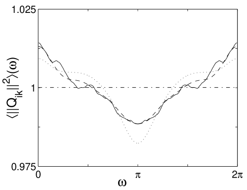
Figure 10: Comparison of averaged overlaps (solid) with semiclassical predictions for the baker map on the sphere (full coupling): approximate resonances (dashed) and traces (dotted). Although the deviation from RMT (dashed-dotted) is small, semiclassical predictions coincide with the quantum result. Only at $\omega=\pi$ the prediction calculated from traces differs slightly. A single Lorentzian peak cannot be observed. Since all resonances have moduli smaller than $\frac{1}{2}$, the corresponding Lorentzians are widely distributed over the interval.

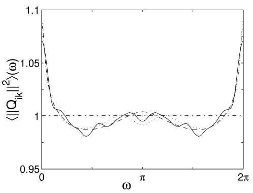
Figure 11: The averaged overlaps and semiclassical predictions for the positive coupling (cf. Fig. 10). At $\omega=0$ we see a Lorentzian peak associated to the resonance resulting from small coupling. The peak heights for the three cases are nearly equal.

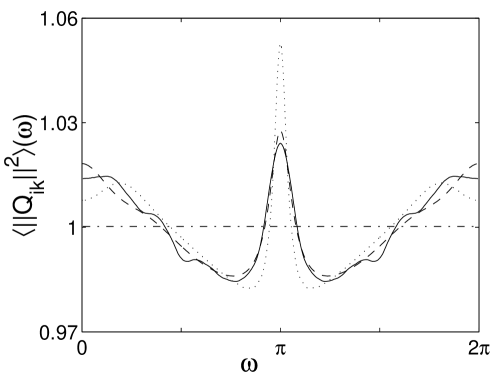
Figure 12: The averaged overlaps and semiclassical predictions for the negative coupling (cf. Fig. 10). The quantum result and the semiclassical prediction from approximate resonances coincide, while the peak corresponding to the coupling resonance is much sharper for the prediction from traces calculated with the use of periodic orbits. This is due to the fact that the approximate resonance in question has not reached the final resonance position which is calculated analytically (cf. Sec. II.2). Quantum uncertainty and noise seem to have the same coarse-graining effect.

As in the classical case Sec. II.4 we here consider three systems: baker map on the sphere and its modifications with positive and negative coupling. For all cases we compare our quantum results with both classical predictions, calculated from approximate resonances and from the traces of the Frobenius–Perron operator obtained with the use of periodic orbits, see Fig. 10–12. The averaged overlaps are scaled such that the RMT average is equal to unity. Up to small fluctuations most of the quantum results coincide with the semiclassical predictions. However, not for every system the quality of the agreement between the semiclassical prediction and the quantum results is the same. Whereas the agreement is fine for the system with positive coupling, the mean resonant peak of the Husimi overlaps approximated by periodic orbits for system (3) is higher than the peak observed in the quantum results, see Fig. 12. On the other hand, the prediction derived by classical resonances obtained by the weak noise approach approximate well the quantum results for all systems studied. In other words, quantum uncertainty acts similarly as a stochastic perturbation of the classical system.

V Coupled Random Matrices – Simplification of the Model

As it has been explained in the foregoing sections the exchange of probability between the two hemispheres is responsible for a resonance. We here study a simplification of the system of coupled baker maps. The internal dynamics, i.e. the baker maps itself, and their corresponding resonances are not the point of interest here. Therefore we replace the quantized baker maps (i.e. the operators (17) and (18)) by random matrices. This simplification might be motivated as follows. Consider a strongly chaotic classical system for which all classical correlations become arbitrary small already after one iteration of the map. Quantizing such a system we expect a random-matrix like behaviour, since all resonances should be located close to the origin and therefore no semiclassical corrections will appear. A realization of such a system can be constructed by a sequence of several uncoupled baker maps $\tilde{B}^{k}$ (Lyapunov exponent $\approx\ln 2^{k}$) followed by a coupling operator. In contrast to the coupled baker maps the coupled random matrices (CRM) are more advantageous. The resonances are easy to calculate as it will be shown in the sequel. Moreover, we have the opportunity to average over an ensemble of arbitrary many coupled random matrices.

For the classical counterpart of CRM we separate the phase space into two partitions of equal area. On the sphere we may choose the northern and southern hemisphere. A strongly chaotic dynamics acts separately on each hemisphere. The classical system can be described by stochastic matrices. To that end we separate the phase space into $2K$ cells, where we conveniently choose $K$ sectors of same area on each hemisphere, for instance $1\dots K$ for the northern and $K+1\dots 2K$ for the southern hemisphere, see Fig. 13a. For the $l$–th cell we define a characteristic (normalized) density function $\mbox{$|\!\!|$}l\mbox{\bf)}$ which is constant inside the cell and vanishes outside. The matrix $A^{(2K)}$ is designed to mimic the FP operator $P$ in this basis

$$A_{il}^{(2K)}=\mbox{\bf(}i\mbox{$|\!\!|$}P\mbox{$|\!\!|$}l\mbox{\bf)}\,.$$ (34)

This is indeed some kind of coarse graining of the Frobenius–Perron operator analogous to the Ulam method for the classical system. For a strongly chaotic dynamics the matrix elements fluctuate around $\frac{1}{K}$, but in this simplification these fluctuations will be neglected. Thus the matrix of the uncoupled system $A_{0}^{(2K)}$ becomes

$$A^{(2K)}_{0}=\left(\begin{array}[]{cc}w^{(K)}&0\\ 0&w^{(K)}\end{array}\right)\,,$$ (35)

where $w_{ik}^{(K)}=\frac{1}{K}$. The eigenvalues of this matrix are easily calculated as $(1,1,0,\dots,0)$, where the degeneracy of eigenvalue $1$ is due to the disjoint invariant densities on each hemisphere.

Figure 13: (a) The sphere is partitioned into $2K$ sectors. (b) A rotation of the sphere permutes the sectors. Here the angle $\Theta$ coincides with one sector for simplicity.

To generate a non-zero resonance we introduce a coupling between both hemispheres as a rotation of the sphere by $\Theta$ around the $x$ axis (perpendicular to the plane of Fig. 13). The system size is chosen that $\frac{\Theta}{2\pi}2K=k$ is integer. In this representation the rotation becomes a $k$-fold cyclic permutation of the cells. Then the (coupled) system is described by

$$A_{\Theta}^{(2K)}=C_{\Theta}^{(2K)}A_{0}^{(2K)}\,,$$ (36)

where $C_{\Theta}^{(2K)}$ is a permutation matrix acting as $i\rightarrow i=i+k\bmod 2K$, see Fig. 13b. A $k$-fold permutation of cells acts on the block-diagonal matrix like a $k$-fold shift of the row vectors, where the trace of this matrix changes for each permutation by $-\frac{2}{K}$ as long as $k$ is smaller than $K$. The eigenvalues of this shifted matrix are easily calculated. Since the matrix is still of rank 2, $2K-2$ eigenvalues are equal to zero. One eigenvalue must be 1, because the matrix is double stochastic. Thus the missing eigenvalue can be calculated from the trace as $\lambda_{1}={\rm tr}A^{(2K)}-1$. Finally the eigenvalue becomes $\lambda_{1}=\frac{2K-2k}{K}-1=1-\frac{2\Theta}{\pi}$.

By varying the rotation angle $\Theta$ the second resonance is controllable over the range $[-1,1]$. For $\Theta=0$ the eigenvalue $1$ is degenerated, since we have two uncoupled systems. A rotation with $\Theta=\frac{\pi}{2}$ mixes both sides uniformly, such that the resonance goes to 0. Finally, choosing $\Theta=\pi$ the hemispheres exchange completely after one map, whereby the resonance becomes $-1$.

The quantization of such a system is easily done. The separated chaotic dynamics on each hemisphere correspond to a Floquet matrix which is block diagonal in the usual $|j,m\rangle$ basis. Due to the phase-space partition we use even dimensions of the Hilbert space, otherwise we are not able to assign the state $|j,m=0\rangle$ to one of the hemispheres. The block matrices are chosen as random unitary matrices due to the strongly chaotic dynamics. The coupling becomes a rotation matrix $R_{x}(\Theta)=e^{-i\Theta\hat{J}_{x}}$

$$U=R_{x}(\Theta)\left(\begin{array}[]{cc}U_{1}&0\\ 0&U_{2}\end{array}\right)\,,$$ (37)

and $U_{1,2}$ are independent random unitary matrices distributed according to the Haar measure on $U(N/2)$.

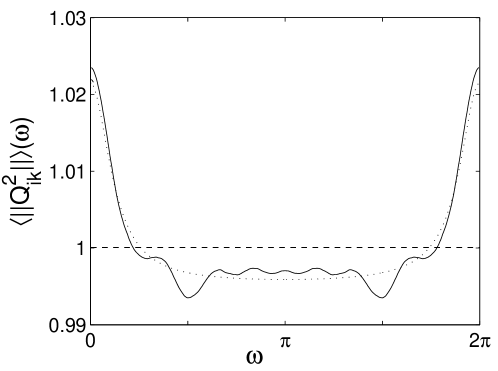
Figure 14: Comparison of averaged overlaps with the semiclassical prediction for CRM with positive coupling. For the quantum results (solid) we find good agreement with the semiclassical prediction (dotted). Uniform spectrum predicted by RMT is denoted by a dashed line.

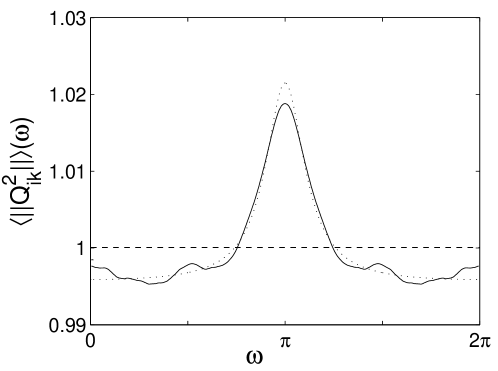
Figure 15: Averaged overlaps of CRM and semiclassical prediction for negative coupling (cf. Fig. 14).

We choose two different coupling angles $\Theta=0.5$ and $\Theta=\pi+0.5$, where the resonances become $\lambda_{\pm}=\pm(1-\frac{1}{\pi})$, respectively. For each case the Hilbert space dimension is $N=200$. Due to the semiclassical prediction the averaged overlaps distribute as

$$\left\langle||Q_{ik}||^{2}\right\rangle(\omega)\propto 1+\frac{1}{N-1}\sum_{n=1}^{\infty}\lambda_{\pm}^{n}\cos(n\omega)\,.$$ (38)

As in the case of the coupled baker maps we use the smoothing with a sinc function of form $\sin(10\omega)/\omega$. Fig. 14 shows the averaged overlaps, $\left\langle||Q_{ik}||^{2}\right\rangle(\omega)$, for the positive resonance $\lambda_{+}$, while in Fig. 15 we see the results for the negative resonance $\lambda_{-}$. For both cases we find a good agreement with the semiclassical prediction. The small fluctuations (much smaller than the Lorentz peaks) of the quantum results are non-generic, i.e. they look different if one chooses other pairs of random matrices.

Concluding remarks

We investigate classical systems whose Frobenius-Perron operators have resonances with large moduli. Such long-lived excitations have a strong impact on the corresponding quantum dynamics. In particular, they constitute a scarring mechanism for quantum eigenfunctions.

In order to detect resonances we employed the small-additive-noise approach. The noise was designed such as to ensure a finite-dimensional representation of the Frobenius-Perron operator which has a unique discrete spectrum.

Our models are chosen such that the classical dynamics is well understood — their topological and metric entropies are both equal to $\ln 2$. For all maps analyzed we provide Markov partitions, as well as the complete sets of periodic orbits. Making use of them we could evaluate the classical Cvitanovic̀-Eckhardt trace formula for the Frobenius-Perron operator cvit2 and discuss its relation to the quantum return probabilities with respect to coherent states. That return probability naturally leads to an intimate relation between long-lived classical resonances and quantum scars. In fact, system specific quantum localization properties not explained by the standard ensembles of random matrices turn out interpretable statistically on the basis of classical Ruelle-Pollicott resonances.

Appendix A Exemplary transition matrices

We present here the transition matrices defined in Sec. II.2 for system (2) and (3) for coupling parameter $\Delta=1/8$. Assuming the lexicographical ordering of cells (that is $A_{1},A_{2},B_{1},B_{2},\ldots$) the transition matrix $\mathbf{T^{+}}$ for the system (2) with positive coupling is equal

$$\mathbf{T^{+}}=\frac{1}{8}\left(\begin{array}[]{*{8}{c}}0&4&0&4&0&0&0&0\\ 4&0&4&0&0&0&0&0\\ 0&0&0&0&8&0&0&0\\ 0&0&0&0&0&8&0&0\\ 0&0&0&0&0&0&8&0\\ 0&0&0&0&0&0&0&8\\ 1&0&1&0&2&0&4&0\\ 0&1&0&1&0&2&0&4\end{array}\right)\ ,$$ (39)

while for the negative coupling (3) it reads

$$\mathbf{T^{-}}=\frac{1}{8}\left(\begin{array}[]{*{8}{c}}0&4&0&2&0&1&0&1\\ 4&0&2&0&1&0&1&0\\ 0&8&0&0&0&0&0&0\\ 8&0&0&0&0&0&0&0\\ 0&0&0&8&0&0&0&0\\ 0&0&8&0&0&0&0&0\\ 0&0&0&0&4&0&4&0\\ 0&0&0&0&0&4&0&4\end{array}\right)\ .$$ (40)

It is straightforward to calculate their eigenvalues and in particular one gets that the second largest eigenvalue in the case of positive coupling (39) is equal $\lambda_{2}^{+}=\frac{a}{6}+\frac{1}{a}\approx 0.8846$ where $a=\sqrt[3]{27+3\sqrt{57}}$, while in the case of negative coupling (40) one has $\lambda_{2}^{-}=-\lambda_{2}^{+}$.

Appendix B Contribution of poles to the traces of FP operator

In order to evaluate the contribution to the trace formula (10) of the poles we first consider stereographic projections of their neighborhoods. In case of the north pole we use stereographic projection from the south pole and vice versa so that in each case the pole corresponds to the origin of the plane. Next we introduce coordinate system such that the discontinuity line of both points corresponds to the negative $x$ axis. Using polar coordinates with $\varphi\in[-\pi,\pi]$ we can easily express the action of the map (the behaviour around the poles of the “positive” and “negative” version is the same) and the mapping around the north pole is given by

$$\left\{\begin{array}[]{c}\varphi\longrightarrow\varphi^{\prime}=\varphi/2+\pi\\ r\longrightarrow r^{\prime}=\sqrt{2}\,r\end{array}\right.\ ,$$ (41)

while for the south pole it reads

$$\left\{\begin{array}[]{c}\varphi\longrightarrow\varphi^{\prime}=\varphi/2\\ r\longrightarrow r^{\prime}=\sqrt{2}\,r\end{array}\right.\ .$$ (42)

The action of these maps is presented in Fig. 16.

Figure 16: The evolution of the phase space around the north and south poles governed by the maps (41) and (42) — top and bottom row, respectively.

From these equations it is clear that the expression (10) is not well defined at the poles. In order to regularize it we replace the $\delta$ function with a two-dimensional Gaussian of width $\sigma$, compute the integral and later go to the limit $\sigma\rightarrow 0$. To this end we need square of the distance between the initial point and its $n$-th iteration

$$d^{2}(r,\varphi)=r^{2}\left[1+2^{n}\mp 2(\sqrt{2})^{n}\cos(1-2^{-n})\varphi\right]$$ (43)

where the upper and lower sign is for the north and south pole, respectively. Putting it all together we get that the contribution to the trace of $P^{n}$ coming from the pole is

$$\lim_{\sigma\rightarrow 0}\frac{1}{2\pi\sigma^{2}}\int_{-\pi}^{\pi}{\rm d}\varphi\int_{0}^{\infty}{\rm d}r\,r\exp\left(-\frac{d^{2}(r,\varphi)}{2\sigma^{2}}\right)\ .$$ (44)

Performing first the radial integral we get

$$\frac{1}{2\pi}\int_{-\pi}^{\pi}{\rm d}\varphi\frac{1}{1+2^{n}\mp 2(\sqrt{2})^{n}\cos(1-2^{-n})\varphi}$$ (45)

which does not depend on the width $\sigma$. Hence the limit $\sigma\rightarrow 0$ is automatically obtained. The integral (45) is elementary and one gets the following result for the contribution of the poles

$$b_{\mp}(n)=\frac{2}{\pi}\frac{2^{n}}{(2^{n}-1)^{2}}\arctan\left(\frac{(\sqrt{2})^{n}\mp 1}{(\sqrt{2})^{n}\pm 1}\tan(1-2^{-n})\frac{\pi}{2}\right)$$ (46)

where the upper and lower sign is for the north and the south pole, respectively. If one compares the above values with the contributions of unstable and inverse unstable fixpoints then one finds that the south pole can be nearly treated like the unstable fixpoint while the north pole differs a bit from the inverse unstable one. To get explicitly the expression (10) for the traces one has to count the number of periodic points using the connectivity matrix $\mathsf{T}$. For instance, for map (3) we obtain

$$\mathop{\operator@font tr}P^{n}=\frac{\mathop{\operator@font tr}(\mathsf{T^{-}})^{n}-4-2(-1)^{n}}{2^{n}+2^{-n}-2}+b_{+}(n)+b_{-}(n)\ ,$$ (47)

where we used (6) and taken into account that Markov partition does not feel the topology of the system (the lines $t=\cos\theta=\pm 1$ are single points — poles) and also the period two orbit originating from $\varphi=\pi$ and $t=-1/3$ is counted twice (see Sec. II.2 and also left hand side of the Fig. 8). Analogously for map (2) we have

$$\mathop{\operator@font tr}P^{n}=\frac{\mathop{\operator@font tr}(\mathsf{T^{+}})^{n}-3-(-1)^{n}}{2^{n}+2^{-n}-2}+b_{+}(n)+b_{-}(n)\ .$$ (48)

In case of the standard baker map on the sphere ($\Delta=1/2$ case of maps (2) and (3)) we are able to find the analytical expression for the number of periodic points so the traces of FP operator are given by

$$\mathop{\operator@font tr}P^{n}=\frac{2^{n}-3-(-1)^{n}}{2^{n}+2^{-n}-2}+b_{+}(n)+b_{-}(n)\ .$$ (49)

References

- (1) A. V. Andreev and B. L. Altshuler, Phys. Rev. Lett. 75 (1995) 902; A. V. Andreev, O. Agam, B. D. Simons, and B. L. Altshuler, Phys. Rev. Lett. 76 (1996) 3947
- (2) M. R. Zirnbauer in: I. V. Lerner, J. P. Keating, and D. E. Khmelnitskii (eds.), Supersymmetry and Trace Formulae: Chaos and Disorder (Kluwer Academic, New York, 1999)
- (3) K. Pance, W. Lu, S. Sridhar, Phys. Rev. Lett. 85, 2737 (2000)
- (4) C. Manderfeld, J. Weber and F. Haake, J. Phys. A 34 (2001) 9893
- (5) D. Ruelle, Phys. Rev. Lett. 56 (1986) 405
- (6) M. Pollicott, Invent. Math. 85 (1986) 147
- (7) P. Gaspard, Chaos, Scattering and Statistical Mechanics, Cambridge University Press 1998
- (8) F. Haake, Quantum Signatures of Chaos, 2nd ed. Springer–Verlag, Heidelberg 2001
- (9) P. Cvitanović, R. Artuso, R. Mainieri, G. Tanner and G. Vattay, Classical and Quantum Chaos, http://www.nbi.dk/ChaosBook/, Niels Bohr Institute (Copenhagen 2001)
- (10) S. Nonnenmacher, http://www.arXiv.org/ e-print archive nlin.CD/0301014
- (11) V. I. Arnold, A. Avez, Ergodic Problems of Classical Mechanics, W. A. Benjamin, New York 1968
- (12) P. Pakoński, A. Ostruszka, K. Życzkowski, Nonlinearity 12 (1999) 269
- (13) A. Ostruszka, P. Pakoński, W. Słomczyński, K. Życzkowski, Phys. Rev. E 62 (2000) 2018
- (14) M. Khodas, S. Fishman, Phys. Rev. Lett. 84 (2000) 2837
- (15) J. Weber, F. Haake and P. Šeba, Phys. Rev. Lett. 85 (2000) 3620
- (16) A. Ostruszka, K. Życzkowski, Phys. Lett. A 289 (2001) 306
- (17) J. Weber, F. Haake, P. A. Braun, C. Manderfeld and P. Šeba, J. Phys. A 34 (2001) 7195
- (18) J. M. Radcliffe, J. Phys. A 4 (1971) 313
- (19) F. T. Arecchi, E. Courtens, R. Gilmore, H. Thomas, Phys. Rev. A 6 (1972) 2211
- (20) R. Glauber and F. Haake, Phys. Rev. A 13 (1976) 357
- (21) A. M. Peremolov, Generalized Coherent States and Their Applications (Springer, New York, 1986)
- (22) N. L. Balazs, A. Voros, Ann. Phys. 190 (1989) 1
- (23) E. J. Heller, Phys. Rev. Lett. 53 (1984) 1515
- (24) E. J. Heller, in Quantum Chaos and Statistical Nuclear Physics (Lecture Notes in Physics 263, ed. T. H. Seligmann and H. Nishioka, Springer–Verlag, Berlin 1986)
- (25) E. J. Heller, Phys. Rev. A 35 (1987) 1360
- (26) M. Kuś, J. Zakrzewski, K. Życzkowski, Phys. Rev. A 43 (1991) 4244
- (27) H.-J. Stöckmann, Quantum Chaos, An Introduction, Cambridge University Press 1999
- (28) C. Manderfeld, J. Phys. A 36 (2003) 6379
- (29) P. Cvitanović and B. Eckhardt, J. Phys. A 24 (1991) L237