The decay of homogeneous anisotropic turbulence

Abstract

We present the results of a numerical investigation of three-dimensional decaying turbulence with statistically homogeneous and anisotropic initial conditions. We show that at large times, in the inertial range of scales: (i) isotropic velocity fluctuations decay self-similarly at an algebraic rate which can be obtained by dimensional arguments; (ii) the ratio of anisotropic to isotropic fluctuations of a given intensity falls off in time as a power law, with an exponent approximately independent of the strength of the fluctuation; (iii) the decay of anisotropic fluctuations is not self-similar, their statistics becoming more and more intermittent as time elapses. We also investigate the early stages of the decay. The different short-time behavior observed in two experiments differing by the phase organization of their initial conditions gives a new hunch on the degree of universality of small-scale turbulence statistics, i.e. its independence of the conditions at large scales.

I Introduction

Decaying turbulence has attracted the attention of various communities and is often considered in experimental, numerical and theoretical investigations [1, 2, 3]. It is in fact quite common that even experiments aimed at studying stationary properties of turbulence involve processes of decay. Important examples are provided by a turbulent flow behind a grid (see [4] and references therein) or the turbulent flow created at the sudden stop of a grid periodically oscillating within a bounded box [5]. In the former case, turbulence is slowly decaying going farther and farther away from the grid and its characteristic scale becomes larger and larger (see [4] for a thorough experimental investigation). Whenever there is sufficient separation between the grid-size $L_{in}$ and the scale of the tunnel or the tank $L_{0}\gg L_{in}$, a series of interesting phenomenological predictions can be derived. For example, the decay of the two-point velocity correlation function, for both isotropic and anisotropic flows, can be obtained under the so-called self-preservation hypothesis (see [3] chapter XVI). That posits the existence of rescaling functions allowing to relate correlation functions at different spatial and temporal scales. By inserting this assumption into the equations of motion, asymptotic results can be obtained both for the final viscosity-dominated regime and for the intermediate asymptotics when nonlinear effects still play an important role.
The status of the self-preservation hypothesis and the properties of energy decay in unbounded flows are still controversial [2, 3, 6, 4]. Systematic results on related problems have been established recently, e.g. for non-linear models of Navier-Stokes equations as Burgers’ equation, see e.g. [7], and for stochastic models of linear passive advection [8], both in unbounded [9, 10, 11, 12] and bounded domains [13, 14].
Here, we investigate the decay of three-dimensional homogeneous and anisotropic turbulence by direct numerical simulations of the Navier-Stokes equations in a periodic box. Previous numerical studies have been limited to either homogeneous and isotropic turbulence [15, 16] or to shell models of the energy cascade [17].
The initial conditions are taken from the stationary ensemble of a turbulent flow forced by a strongly anisotropic input [18]. The correlation lengthscale of the initial velocity field $L_{in}$ is of the order of the size of the box $L_{0}\approx L_{in}$.
In the first part of this paper, we shall try to answer the following questions about the intermediate asymptotic regime of nonlinear decay: How do global quantities, such as single-point velocity and vorticity correlations, decay ? What is the effect of the outer boundary on the decay laws ? Do those quantities keep track of the initial anisotropy ? As for the statistics of velocity differences within the inertial range of scales, is there a recovery of isotropy at large times ? If so, do strong fluctuations get isotropic at a faster/slower rate with respect to those of average intensity ? Do isotropic and anisotropic fluctuations decay self-similarly ? If not, do strong fluctuations decay slower or faster than typical ones ?
In the second part we study the early stages of the decay, with the aim of establishing a link between the small-scale velocity statistics in this phase and in the forced case. That will allow us to argue in favor of an “exponents only” universality scenario, for forced hydrodynamic turbulence.

II Numerical setup

A The initial conditions

The initial conditions are taken from the stationary ensemble of a forced random Kolmogorov flow [18]. For sake of completeness, we recall here some of the statistical properties of this forced turbulent flow. We consider the solutions of the Navier-Stokes equations for an incompressible velocity field $v$.

$$\partial_{t}{{\mbox{\boldmath$v$}}}+({{\mbox{\boldmath$v$}}}\cdot{\bf\nabla}){{\mbox{\boldmath$v$}}}=-{\bf\nabla}p+\nu\Delta{{\mbox{\boldmath$v$}}},$$ (1)

in a three-dimensional periodic domain. To maintain a statistically stationary state Eq. (1) had to be supplemented by an input term $f$ acting at large scales. This force was strongly anisotropic: ${{\mbox{\boldmath$f$}}}=(0,0,f_{z}(x))$ with $f_{z}(x)=F_{1}\cos[2\pi x/L_{x}+\phi_{1}(t)]+F_{2}\cos[4\pi x/L_{x}+\phi_{2}(t)]$, constant amplitudes $F_{1,2}$ and independent, uniformly distributed, $\delta$-correlated in time random phases $\phi_{1,2}(t)$. This choice ensured the statistical homogeneity of the forcing and thus of the velocity field. We simulated the forced random Kolmogorov flow at resolution $256^{3}$ for time spans up to $70$ eddy turnover times [18]. The viscous term was replaced by a second-order hyperviscous term $-\nu\Delta^{2}{{\mbox{\boldmath$v$}}}$. We stored $40$ statistically independent configurations that here serve as initial conditions for the decaying runs.

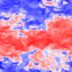
(a) $v_{z}(\tau_{0})$

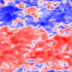
(b) $v_{z}(10\tau_{0})$

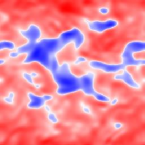
(c) $v_{z}(100\tau_{0})$

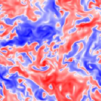
(d) $v_{x}(\tau_{0})$

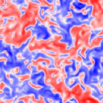
(e) $v_{x}(10\tau_{0})$

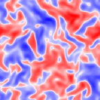
(f) $v_{x}(100\tau_{0})$

FIG. 1.: Two-dimensional sections of a typical velocity field at different times of decay. The three top images and the three bottoms are the grayscale plots of the velocity components parallel and transverse to the direction of the forcing, respectively. Note in the upper row, the presence of anisotropic structures which decay as time elapses.

B Decaying runs

As turbulence decays, the effective Reynolds number $Re=v_{rms}L_{0}/\nu$ decreases, while the viscous characteristic scale and time increase. To speed up the numerical time-marching, it is then convenient to use an adaptative scheme. We calculate periodically the smallest eddy-turnover time from the energy spectrum and set the time step as $1/100$ thereof. The whole velocity-field configuration is then dumped for offline analysis at fixed multiples $\{0,1,10,10^{2},10^{3},10^{4},10^{5},10^{6}\}\,\tau_{0}$ of the initial large-scale eddy turnover time $\tau_{0}=L_{0}/v_{rms}^{t=0}$. In Fig. 1 we show a two dimensional section in the plane $x$-$z$ of the velocity components $v_{z}$ and $v_{x}$.

III The decay of global quantities

A first hint on the restoration of isotropy at large times can be obtained by the two-dimensional snapshots in Fig. 1. After a few eddy turnover times, it is evident that large-scale fluctuations become more and more isotropic. To give a quantitative measure, we collect for each run the temporal behavior of the following one-point quantities:

$$E_{ij}={\overline{v_{i}(t)v_{j}(t)}},$$ (2)

$$\Omega_{ij}={\overline{\omega_{i}(t)\omega_{j}(t)}}.$$ (3)

By $\overline{\cdots}$ we denote the average over space coordinates only, whereas $\left\langle\cdots\right\rangle$ will indicate the average over both initial conditions and space. The symmetric matrices $E_{ij}(t)$ and $\Omega_{ij}(t)$ are then diagonalized at each time-step and the eigenvalues $E_{1}(t),E_{2}(t),E_{3}(t)$ and $\Omega_{1}(t),\Omega_{2}(t),\Omega_{3}(t)$ are extracted. Since the forcing points in a fixed direction two eigenvalues are almost degenerate, say $E_{2}$ and $E_{3}$, and strongly differ from the first one, $E_{1}$. The typical decay of $E_{i}(t)$ and $\Omega_{i}(t)$ for $i=1,\dots,3$ is shown in Fig. 2. During the self-similar stage, $t\in[10,10^{6}]$, the energy eigenvalues fall off as $E_{\{1,2,3\}}\sim t^{-2}$, as expected for the decay in a bounded domain [4, 15]. The enstrophy eigenvalues, $\Omega_{\{1,2,3\}}$ decay as $t^{-12/5}$. The dimensional argument that captures these algebraic laws proceeds as follows. The energy decay is obtained by the energy balance $dE(t)/dt=-\epsilon(t)$, where we estimate $E\sim v_{rms}^{2}(t)$ and $\epsilon(t)\sim v_{rms}^{3}(t)/L_{0}\sim E^{3/2}(t)/L_{0}$, and obtain $E(t)\sim t^{-2}$ and $\epsilon(t)\sim t^{-3}$. As for the vorticity decay, we have $\Omega(t)\sim(\delta_{\eta}v)^{2}/\eta^{2}$, where $\eta$ is the dissipative lengthscale and $\delta_{\eta}v$ is the typical velocity difference at separation $\eta$. Assuming a Kolmogorov scaling $\delta_{\eta}v\sim\epsilon(t)^{1/3}\eta^{1/3}$, and recalling that for a second-order hyperviscous dissipation $\epsilon(t)\sim\nu(\delta_{\eta}v)^{2}/\eta^{4}$ we obtain $\eta\sim t^{3/10}$ and $\delta_{\eta}v\sim t^{-9/10}$, whence $\Omega(t)\sim t^{-12/5}$. We now focus on the process of recovery of isotropy in terms of global quantities. We identify two set of observables

$$\Delta_{ij}E(t) = \left\langle{E_{i}(t)-E_{j}(t)}\over{E_{i}(t)+E_{j}(t)}\right\rangle\,,$$ (4)

$$\Delta_{ij}{\Omega}(t) = \left\langle{\Omega_{i}(t)-\Omega_{j}(t)}\over{\Omega_{i}(t)+\Omega_{j}(t)}\right\rangle\,,$$ (5)

which vanish for isotropic statistics. Their rate of decay is therefore a direct measurement of the return to isotropy. The energy matrix $E_{ij}$ is particularly sensitive to the large scales while small-scale fluctuations are sampled by $\Omega_{ij}$. As it can be seen from Fig. 3, both large and small scales begin to isotropize after roughly one eddy turnover time and become fully isotropic (within statistical fluctuations) after $100$ eddy turnover times. However, small scales show an overall degree of anisotropy much smaller than the large scales.

FIG. 2.: Log-log plot of the eigenvalues of energy and vorticity matrices vs. time, expressed in $\tau_{0}$ unit.

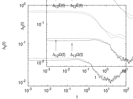
FIG. 3.: Log-log plot of the anisotropy content at the large scales ($\Delta_{12}E(t)$, $\Delta_{13}E(t)$, top curves) and the small scales ($\Delta_{12}\Omega(t)$, $\Delta_{13}\Omega(t)$, bottom curves) as a function of time, expressed in $\tau_{0}$ unit. The large-scale (small-scale) anisotropy content is defined as the mismatch between the eigenvalues of the single-point velocity (vorticity) correlation.

IV The decay of small-scale fluctuations

A The self-preservation hypothesis for anisotropic decay

The observables which characterize the decay of small-scale velocity fluctuations are the longitudinal structure functions

$$S^{(n)}\left({\bf r},t\right)=\left\langle\left[\left({\mbox{\boldmath$v$}}\left({\mbox{\boldmath$x$}}+{\bf r},t\right)-{\mbox{\boldmath$v$}}\left({\mbox{\boldmath$x$}},t\right)\right)\cdot\hat{\bf r}\right]^{n}\right\rangle\,.$$ (6)

Those quantities depend not only on the modulus of the separation ${\bf r}$ but also on its orientation $\hat{\bf r}$, since the velocity statistics is anisotropic. A method to systematically disentangle isotropic from anisotropic contributions in the structure functions is based on the irreducible representations of the SO(3) group [19]. In this approach, the observables (6) are expanded on the complete basis of the eigenfunctions of the rotation operator. The SO(3) decomposition of scalar objects, such as structure functions, is obtained by projection on the spherical harmonics $Y_{jm}({\mbox{\boldmath$\hat{r}$}})$:

$$S^{(n)}({\bf r},t)=\sum_{j=0}^{\infty}\sum_{m=-j}^{j}S^{(n)}_{jm}\left(r,t\right)Y_{jm}({\mbox{\boldmath$\hat{r}$}}).$$ (7)

Here, $S^{(n)}_{jm}\left(r,t\right)$ denotes the projection of the $n$-th order structure function on the $(j,m)$ SO(3) sector, with $j$ and $m$ labeling the total angular momentum and its projection in the direction $\hat{z}$, respectively. Another equivalent possibility is to look at the SO(3) decomposition of the PDF of the longitudinal velocity differences. In this case, denoting by ${\cal P}(\Delta,{\bf r};t)$ the probability that the longitudinal incremement ${\delta_{r}v}\equiv\left({\mbox{\boldmath$v$}}({\bf r},t)-{\mbox{\boldmath$v$}}(0,t)\right)\cdot{\mbox{\boldmath$\hat{r}$}}$ be equal to $\Delta$, we may project ${\cal P}(\Delta,{\bf r};t)$ on the SO(3) basis:

$${\cal P}(\Delta,{\bf r};t)=\sum_{j=0}^{\infty}\sum_{m=-j}^{j}{\cal P}_{jm}\left(r,\Delta;t\right)Y_{jm}({\mbox{\boldmath$\hat{r}$}}).$$ (8)

The projection ${\cal P}_{jm}\left(r,\Delta;t\right)$ plays the role of an “effective PDF” for each single SO(3) sector. (It should be however remarked that only the isotropic probability density ${\cal P}_{00}\left(r,\Delta;t\right)$ has the property of being everywhere positive and normalized to unity with respect to the weight $r^{2}/(4\pi)$.) Indeed, the projections of the longitudinal structure function on any sector $(j,m)$ can be reconstructed from the corresponding ${\cal P}_{jm}\left(r,\Delta;t\right)$ by averaging over all possible $\Delta$’s:

$$S^{(n)}_{jm}\left(r,t\right)=\int d\Delta\Delta^{n}{\cal P}_{jm}\left(r,\Delta;t\right)\,.$$ (9)

That establishes the equivalence between the decompositions (7) and (8).
The main points broached here are about the long-time properties of the SO(3) projections, $S^{(n)}_{jm}\left(r,t\right)$. A simple isotropic generalization of the self-preservation hypothesis (see, e.g. Ref. [2]) amounts to writing:

$$S^{(n)}_{jm}\left(r,t\right)=V^{(n)}_{jm}\left(t\right)f^{(n)}_{jm}\left(r/L_{jm}(t)\right).$$ (10)

Note that $V^{(n)}_{jm}\left(t\right)$ takes explicitly into account the fact that large-scale properties may depend in a nontrivial way on both $(j,m)$ and the order $n$. Furthermore, $L_{jm}(t)$ accounts for the possibility that the characteristic length scale depend on the SO(3) sector.
In analogy with the observations made in the stationary case [20, 21, 22, 23, 18, 24, 25, 26] we postulate a scaling behavior

$$S^{(n)}_{jm}\left(r,t\right)\sim a^{(n)}_{jm}(t)\left(\frac{r}{L_{jm}(t)}\right)^{\zeta_{j}^{(n)}}\,.$$ (11)

The time behavior is encoded in both the decay of the overall intensity, accounted by the prefactors $a^{(n)}_{jm}(t)$, and the variation of the integral scales $L_{jm}(t)$. The representation (11) is the simplest one fitting the initial time statistics for $t=0$ and agreeing with the evolution given by the self preservation hypothesis in the isotropic case. The power law behavior for $f^{(n)}_{jm}\left(r/L_{jm}(t)\right)$ can be expected only in a time-dependent inertial range of scales $\eta(t)\ll r\ll L(t)$. As for the exponents appearing in (11), their values are expectedly the same as in the stationary case. In the latter situation it has been shown that they are organized hierarchically according to their angular sector $j$ [24] :

$$\zeta_{0}^{(n)}\leq\zeta_{1}^{(n)}\leq\cdots\zeta_{j}^{(n)}\leq\cdots.$$ (12)

Since the isotropic sector has the smallest exponent, at any given time and for a given intensity of the fluctuation (selected by the value of $n$) we have a recovery of isotropy going to smaller and smaller scales. Yet, deviations of the scaling exponents from their dimensional expectations make the recovery at small-scales much slower than what predicted by dimensional analysis [26, 25]. Moreover, there are quantities which should vanish in an isotropic field and actually blow up as the scale decreases [25].
Concerning the time evolution, it seems difficult to disentangle the dependence due to the decay of $a^{(n)}_{jm}(t)$ from the one due to the growth of the integral scale $L_{jm}(t)$. Here, we note only that the existence of a running reference scale, $L_{jm}(t)$ introduces some non-trivial relations between the spatial anomalous scaling and the decaying time properties, and those relations might be subject to experimental verification. In our case, the fact that the initial condition has a characteristic lengthscale comparable with the box size, simplifies the matter. Indeed we expect that $L_{jm}(t)\approx L_{0}$, and the decay is due only to the fall off of the global intensity $a^{(n)}_{jm}(t)$. Unfortunately, a shortcoming is that the width of the inertial range $L_{0}/\eta(t)$ shrinks monotonically in time, thereby limiting the possibility of precise quantitative statements.

B Numerical results

An overall view of the SO(3) projections at all resolved scales and for all measured decay times is presented in Fig. 4 for $n=2$ and the isotropic, $(j=0,m=0)$, sector. The same quantities are presented in Fig. 5 for the most intense anisotropic sector $(j=4,m=0)$.

FIG. 4.: Log-log plot of the isotropic component of the second order projection $S^{(2)}_{00}\left(r,t\right)$ vs. $r$ for $7$ decay times, $t=0,\tau_{0},10\tau_{0},10^{2}\tau_{0},10^{3}\tau_{0},10^{4}\tau_{0},10^{5}\tau_{0}$ (from top to bottom). The two straight lines correspond to the inertial range slope $S^{(2)}_{00}\left(r,t\right)\sim r^{0.7}$ (top) and to the smooth differentiable slope $S^{(2)}_{00}\left(r,t\right)\sim r^{2}$ (bottom).

FIG. 5.: The same quantities as in the previous figure but for the anisotropic sector $j=4,m=0$, i.e. log-log plot of $S^{(2)}_{40}\left(r,t\right)$ vs. $r$.

We notice that as time elapses the dissipative range erodes the inertial one, as a consequence of the growth of the Kolmogorov scale $\eta(t)$. We notice in passing that the two curves corresponding to $t=0$ and $t=\tau_{0}$ almost coincide, i.e. even small scales are unchanged despite their typical eddy turnover times is much smaller than $\tau_{0}$. This finding has some consequences that will be discussed at length in section V. A similar qualitative trend is displayed by the most intense anisotropic sector, $(j=4,m=0)$ shown in Fig. 5, even though oscillations at small scales spoil significantly the scaling properties at small separations $r$.

FIG. 6.: Log-log plot of $S^{(2)}_{jm}\left(r,t\right)$ vs. $r$, at $t=\tau_{0}$. Symbols refer to $(j=0,m=0)$ (top) and to $(j=4,m=0)$ (bottom).

FIG. 7.: The same quantities as in the previous figure but at the later time $t=10^{2}\tau_{0}$. The sectors shown are $(j=0,m=0)$ and $(j=4,m=0)$ (top to bottom), as in the previous figure.

In order to assess the relative importance of isotropic and anisotropic contributions, we plot in Fig. 6 the SO(3) projections of some $(j,m)$ sectors for the order $n=2$ and a fixed time, $t=\tau_{0}$. Fig. 7 shows the same quantities as in Fig. 6 but at a later time, $t=100\tau_{0}$. Although the small-scale behavior of anisotropic sectors readily becomes rather noisy, the various contributions are organized hierarchically and the isotropic contribution is dominant, as expected.
Let us now analyze quantitatively the time-decay of the structure functions at a fixed separation. In Fig. 8 we show the long-time decay of the second and fourth-order moments on the isotropic and an anisotropic sector at $r=80$, within the inertial range.

FIG. 8.: Log-log plot of the second-order moment $S^{(2)}_{jm}\left(r=80,t\right)$ for the isotropic sector $(j=0,m=0)$ and the anisotropic sector $(j=4,m=0)$, vs. time, for a separation $r$ in the inertial range. In the inset we plot the same curves for the fourth-order moment $S^{(4)}_{jm}\left(r=80,t\right)$.

FIG. 9.: Hierarchical organization of anisotropic fluctuations at long times. Log-log plot of the anisotropic projections normalized by the corresponding isotropic projection (see text), at two fixed scales $r=80$ and $r=40$ (inset) for $n=2,4,6$ in the anisotropic sector $j=4,m=0$. Symbols read as follows : $\Pi^{(2)}_{40}$ (full box); $\Pi^{(4)}_{40}$ (star); $\Pi^{(6)}_{40}$ (empty box). The straight line is $t^{-\chi^{*}}$ with $\chi^{*}\sim 0.3$. Same symbols in the inset.

We observe that the anisotropic sectors decay faster than the isotropic one, i.e. at a fixed scale there is a tendency towards the recovery of isotropy at large times. The relative rate of decay can be quantified by the observable

$$\Pi^{(n)}_{jm}\left(r,t\right)\equiv\frac{S^{(n)}_{jm}\left(r,t\right)}{S^{(n)}_{0,0}\left(r,t\right)}\sim t^{-\chi_{j}^{(n)}}\,.$$ (13)

In Fig. 9 we show $\Pi^{(n)}_{jm}\left(r,t\right)$ at $r=80$ for structure functions of order $n=2,4,6$ and for $(4,0)$, one of the most intense anisotropic sectors. In the inset we also plot the same quantities at the smaller scale $r=40$. All anisotropic sectors, for all measured structure functions, decay faster than the isotropic one. The measured slope in the decay is about $\chi_{j}^{(n)}\sim 0.3$ almost independent, within the statistical errors, of the order $n$. Note that these results agree with the simple picture that the time-dependence in (11) is entirely carried by the prefactors $a_{jm}^{(n)}(t)$ and the value of the integral scales $L_{jm}(t)$ is saturated at the size of the box. Indeed, by assuming that large-scale fluctuations are almost Gaussian we have that the leading time-dependency of $a_{jm}^{(2n)}$ is given by $a_{jm}^{(2)}a_{00}^{(2n-2)}$. For the isotropic sector, $a_{00}^{(2n)}\sim(a_{00}^{(2)})^{n}$, and plugging that in (13), we get: $\Pi^{(n)}_{jm}\left(r,t\right)\sim a^{(2)}_{jm}(t)/a^{(2)}_{00}(t)\sim t^{-\chi^{*}}$ with $\chi^{*}\sim 0.3(\pm 0.1)$ independent of $n$. The quality of our data is insufficient to detect possible residual effects due to $L_{jm}(t)$, which would make $\chi_{j}^{(n)}$ depend on $n$ and $j$ because of spatial intermittency.
The interesting fact that we measure decay properties of the anisotropic sectors which are almost independent of the order of the structure functions indicate that we must expect some non-trivial time dependence in the shape of the PDF’s ${\cal P}_{jm}\left(r,\Delta;t\right)$ for $j>0$. The most accurate way to probe the rescaling properties of ${\cal P}_{jm}\left(r,\Delta;t\right)$ in time is to compute the generalized flatness:

$$K_{jm}^{(n)}(r,t)\equiv\frac{S^{(n)}_{jm}\left(r,t\right)}{\left(S^{(2)}_{jm}\left(r,t\right)\right)^{\frac{n}{2}}}\sim t^{\alpha_{j}^{(n)}}$$ (14)

Were the PDF projection in the $(j,m)$ sector self-similar for $t\gg\tau_{0}$, then $K_{jm}^{(n)}(r,t)$ would tend to costant values. This is not the case for anisotropic fluctuations, as it is shown in Fig. (10). The curves $K_{jm}^{(n)}(r,t)$ are collected for two fixed inertial range separations, $r=80$ and $r=40$ (inset), for two different orders, $n=4,6$ and for both the isotropic and one of the most intense anisotropic sectors$(j=4,m=0)$ . The isotropic flatness tends toward a constant value for large $t$. Conversely, its anisotropic counterparts are monotonically increasing with $t$, indicating a tendency for the anisotropic fluctuations to become more and more intermittent as time elapses. A consequence of the monotonic increase of intermittency for large times is the impossibility to find a rescaling function, $g(t,r)$, which makes the rescaled PDF $g(t,r){\cal P}_{jm}\left(r,\frac{\Delta}{g(t,r)};t\right)$ time-independent at large times. Let us notice that also the behavior in Fig. 10 is in qualitative agreement with the observation previously made that all time dependencies can be accounted by the prefactors $a_{jm}^{(n)}(t)$. Indeed, assuming that the length scales $L_{jm}(t)$ have saturated and that the large scale PDF is close to Gaussian, it is easy to work out the prediction $K_{jm}^{(n)}(r,t)\sim t^{-\chi^{*}(1-n/2)}$, i.e. $\alpha_{j}^{(n)}=\chi^{*}(n/2-1)$.

FIG. 10.: Log-log plot of the generalized flatness, $K_{jm}^{(n)}(r,t)$ of order $n=4,6$ for both the isotropic (two bottom curves), and the anisotropic sector $(j=4,m=0)$ (two top curves) at $r=80$, and as a function of time. In the inset we plot the same quantities, in the same order, at a different inertial range scale, $r=40$.

We conclude this section by a brief summary of the results. We have found that isotropic fluctuations persist longer than anisotropic ones, i.e. there is a time-recovery, albeit slower than predicted by dimensional arguments, of isotropy during the decay process. We have also found that isotropic fluctuations decay in an almost self-similar way whilst the anisotropic ones become more and more intermittent. Qualitatively, velocity configurations get more isotropic but anisotropic fluctuations become, in relative terms, more “spiky” than the isotropic ones as time elapses.

V Short-time decay

Let us now move to the properties of decay at short times ($t\ll\tau_{0}$). Universality of small-scale forced turbulence is at the forefront of both theoretical and experimental investigation of real turbulent flows [2]. The problem is to identify those statistical properties which are robust against changes of the large-scale physics, that is against changes in the boundary conditions and the forcing mechanisms. Our goal here is to relate the small-scale universal properties of forced turbulent statistics to those of short-time decay for an ensemble of initial configurations. An immediate remark is that one cannot expect an universal behaviour for all statistical observables as the very existence of anomalous scaling is the signature of the memory of the boundaries and/or the external forcing throughout all the scales. Indeed, the main message we want to convey here is that only the scaling of both isotropic and anisotropic small-scale fluctuations is universal, at least for forcings concentrated at large scales. The prefactors are not expected to be so. There is therefore no reason to expect that quantities such as the skewness, the kurtosis and in fact the whole PDF of velocity increments or gradients be universal.
This is the same behavior as for the passive transport of scalar and vector fields (see [8] and references therein). For those systems both the existence and the origin of the observed anomalous scaling laws have been understood and even calculated analytically for some instances in the special class of Kraichnan flows [27]. Here, it is worth stressing that the universal character of scaling exponents is shared by both isotropic and anisotropic fluctuations [28].
For the Navier-Stokes case we have a huge amount of experimental and numerical indications that the velocity field shows anomalous scaling [2], suggesting the existence of phenomena “similar” to those of the linear case. However, carrying over the analytical knowledge developed for linear hydrodynamical problems involve some nontrivial, yet missing, steps. For the Navier-Stokes dynamics, linear equations of motion surface again but at the functional level of the whole set of correlation functions. In a schematic form:

$$\partial_{t}C^{(n)}=\Gamma^{(n+1)}C^{(n+1)}+\nu D^{(n)}C^{(n)}+F^{(n)},$$ (15)

where $\Gamma^{(n+1)}$ is the integro-differential linear operator coming from the inertial and pressure terms and $C^{(n+1)}$ is a shorthand notation for a generic $(n+1)$-point correlator. The molecular viscosity is denoted by $\nu$ and $D^{(n)}$ is the linear operator describing dissipative effects. Finally, $F^{(n)}$ is the correlator involving increments of the large-scale forcing $f$ and of the velocity field. Balancing inertial and injection terms gives dimensional scaling, and anomalously scaling terms must therefore have a different source. A natural possibility is that a mechanism similar to the one identified in linear transport problems be at work in the Navier-Stokes case as well. The anomalous contributions to the correlators would then be associated to statistically stationary solutions of the unforced equations (15). The scaling exponents would a fortiori be independent of the forcing and thus universal. As for the prefactors, the anomalous scaling exponents are positive and thus the anomalous contributions grow at infinity. They should then be matched at the large scales with the contributions coming from the forcing to ensure that the resulting combination vanish at infinity, as required for correlation functions. Our aim here is not to prove the previous points but rather to check over the most obvious catch: the Navier-Stokes equations being integro-differential, non-local contributions might directly couple inertial and injection scales and spoil the argument. This effect might be particularly relevant for anisotropic fluctuations where infrared divergences may appear in the pressure integrals [29].

FIG. 11.: Top: Temporal decay of the second-order isotropic structure function $S^{(2)}_{00}(r,t)$, rescaled by its value at $t=0$. Here $r=30$, inside the inertial range. The two curves refer to the time evolution of the structure function starting from the forced-stationary velocity fields (squares, set A) and from the randomly dephased velocity fields (circles, set B). Time is normalized by the integral eddy turnover time. Notice that for set B we observe changes on a time scale faster than the integral eddy turnover time. That is to be contrasted with the case A, where structure functions are strictly constant in time up to an integral eddy turnover time. Bottom: The same curves but for the fourth-order structure function.

In order to investigate the previous point, we performed two sets of numerical experiments in decay. The first set, A, is of the same kind as in the previous section, i.e. we integrated the unforced Navier-Stokes equations (1) with initial conditions picked from an ensemble obtained from a forced anisotropic stationary run. Statistical observables are measured as an ensemble average over the different initial conditions, $\langle\bullet\rangle_{ens}$. The ensemble at the initial time of the decay process is therefore coinciding with that at the stationary state in forced runs. If correlation functions are indeed dominated at small scales by statistically stationary solutions of the unforced equations then the field should not decay. Specifically, the field should not vary for times smaller than the large-scale eddy turnover time $\tau_{0}\sim L_{0}/\langle v^{2}\rangle^{1/2}$, with $L_{0}$ denoting the integral scale of the flow. Those are the times when the effects of the forcing terms start to be felt. Note that this should hold at all scales, including the small ones whose turnover times are much faster than $\tau_{0}$. The second set of numerical simulations (set B) is meant to provide for a stringent test of comparison. The initial conditions are the same as before but for the random scrambling of the phases : $\hat{v}_{i}({\mbox{\boldmath$k$}})\rightarrow P_{il}({\mbox{\boldmath$k$}})\,\hat{v}_{l}({\mbox{\boldmath$k$}})\,\exp(i\,\theta_{l}({\mbox{\boldmath$k$}}))$. Here, $\hat{v}$ denotes the Fourier transform and $P_{il}({\mbox{\boldmath$k$}})$ is the incompressibility projector. In this way, the spectrum and its scaling are preserved but the wrong organization of the phases is expected to spoil the statistical stationarity of the initial ensemble. As a consequence, two different decays are expected for the two sets of experiments. In particular, contrary to set A, set B should vary at small scales on times of the order of the eddy turnover times $\tau_{r}\sim r^{2/3}$. This is exactly what we found in the numerical simulations, as can be seen in Fig. 11, where the temporal behavior of longitudinal structure functions of order 2 and 4 is shown. The scaling of the contributions responsible for the observed behaviour at small scales are thus forcing independent.
As for anisotropic fluctuations, we also found two very different behaviors depending on the set of initial conditions. In Fig. 12 we show the case of the projection $S^{(n)}_{jm}(r=60,t)$  for the anisotropic sector $j=4$,$m=0$. As it can be seen, for set A of initial conditions the function is indeed not decaying up to a time of the order of $\tau_{0}$.
To conclude, the data presented here support the conclusion that nonlocal effects peculiar to the Navier-Stokes dynamics do not spoil arguments on universality based on analogies with passive turbulent transport. The picture of the anomalous contributions to the correlation functions having universal scaling exponents and non-universal prefactors follows.

FIG. 12.: The same curves as in the previous figure but for the anisotropic sector $(j=4,m=0)$.

VI Conclusions

We have presented a numerical investigation of the decay of three-dimensional turbulence, both isotropic and anisotropic. Concerning short-time decay, we have compared the decay for two different sets of initial conditions, with and without phase correlations. That gave some new hints on the properties of universality of isotropic and anisotropic forced turbulence. As for long times, we have found that fluctuations in the inertial range become more and more isotropic. On the other hand, the anisotropic components become more and more intermittent, i.e. relatively intense anisotropic fluctuations become more and more probable. The main issue here was to investigate the effects of a bounded domain, i.e. situations where the integral scale cannot grow indefinitely. The decay process at long times is then governed by the set-up at large scales. Anisotropies decay in time at a rate almost independent of the order of the moments and of the kind of anisotropic fluctuations. Projections of the PDF’s on different SO(3) sectors show different intermittent properties (with the anisotropic sectors being more intermittent). An obvious further development of this study would be to investigate the case where the integral scales $L_{jm}(t)$ vary in time. Additional intermittency in time might then be brought in by the anomalous scaling in the space variables of the correlation functions.

This research was supported by the EU under the Grants No. HPRN-CT 2000-00162 “Non Ideal Turbulence” and No. HPRN-CT-2002-00300 ”Fluid Mechanical Stirring and Mixing”, and by the INFM (Iniziativa di Calcolo Parallelo). A.L. acknowledges the hospitality of the Observatoire de la Côte d’Azur, where part of the work has been done.

REFERENCES

- [1] G.K. Batchelor, The Theory of Homogeneous Turbulence, Cambridge University Press, Cambridge (1953).
- [2] U. Frisch, Turbulence: The Legacy of A. N. Kolmogorov, Cambridge University Press, Cambridge (1995).
- [3] A.S. Monin and A.M. Yaglom Statistical Fluid Mechanics, MIT Press, Cambridge MA, (1975).
- [4] L. Skrbek and S.R. Stalp, “On the decay of homogeneous isotropic turbulence,” Phys. Fluids 12, 1997 (2000).
- [5] I.P.D. De Silva and H.J.S. Fernando, “Oscillating grids as a source of nearly isotropic turbulence,” Phys. Fluids 6, 2455 (1994).
- [6] C.G. Speziale and P. Bernard, J. Fluid Mech. 241, 645 (1992).
- [7] U. Frisch and J. Bec, in Les Houches 2000: New Trends in Turbulence eds. M. Lesieur, A.M. Yaglom and F. David, pp. 341, Springer-EDP Sciences, Les Ulis (2001).
- [8] G. Falkovich, K. Gawȩdzki, and M. Vergassola, “Particles and fields in fluid turbulence,” Rev. Mod. Phys. 73, 913 (2001).
- [9] D.T. Son, “Turbulent decay of a passive scalar in the Batchelor limit : exact results from a quantum-mechanical approach,” Phys. Rev. E 59, R3811, (1999).
- [10] E. Balkovsky and A. Fouxon, “Universal long-time properties of Lagrangian statistics in the Batchelor regime and their application to the passive scalar problem,” Phys. Rev. E 60, 4164 (1999).
- [11] G. Eyink and J. Xin, “Self-similar decay in the Kraichnan model of a passive scalar,” J. Stat. Phys. 100, 679 (2000).
- [12] M. Chaves, G. Eyink, U. Frisch, and M. Vergassola, “Universal decay of scalar turbulence,” Phys. Rev. Lett. 86, 2305 (2001).
- [13] M. Chertkov and V. Lebedev, ”Decay of scalar turbulence revisited”, nlin.CD/0209013 (2002).
- [14] J. Sukhatme and R.T. Pierrehumbert, “Decay of passive scalars under the action of single scale smooth velocity fields in bounded two-dimensional domains: From non-self-similar probability distribution functions to self-similar eigenmodes,” Phys. Rev. E 66, 056302 (2002).
- [15] V. Borue and S.A. Orszag, “Self-similar decay of three-dimensional homogeneous turbulence with hyperviscosity,” Phys. Rev. E 51, R856 (1995).
- [16] H. Touil, J.-P. Bertoglio, and L. Shao, Journ. Turb. 3, 49 (2002).
- [17] J-O. Hooghoudt, D. Lohse and F. Toschi, “Decaying and kicked turbulence in a shell model,” Phys. Fluids 13, 2013 (2001).
- [18] L. Biferale and F. Toschi, “Anisotropic Homogeneous Turbulence: Hierarchy and Intermittency of Scaling Exponents in the Anisotropic Sectors,” Phys. Rev. Lett. 86, 4831 (2001).
- [19] I. Arad, V. S. L’vov, and I. Procaccia, “Correlation functions in isotropic and anisotropic turbulence: The role of the symmetry group,” Phys. Rev. E 59, 6753 (1999).
- [20] S. Garg and Z. Warhaft, “On the small scale structure of simple shear flow,” Phys. Fluids 10, 662 (1998).
- [21] I. Arad, B. Dhruva, S. Kurien, V. S. L’vov, I. Procaccia, and K. R. Sreenivasan, “Extraction of Anisotropic Contributions in Turbulent Flows,” Phys. Rev. Lett. 81, 5330 (1998).
- [22] I. Arad, L. Biferale, I. Mazzitelli, and I. Procaccia, “Disentangling Scaling Properties in Anisotropic and Inhomogeneous Turbulence,” Phys. Rev. Lett. 82, 5040 (1999).
- [23] S. Kurien and K. R. Sreenivasan, “Anisotropic scaling contributions to high-order structure functions in high-Reynolds-number turbulence,” Phys. Rev. E 62, 2206 (2000).
- [24] L. Biferale, I. Daumont, A. Lanotte, and F. Toschi, “Anomalous and dimensional scaling in anisotropic turbulence,” Phys. Rev. E 66, 056306 (2002).
- [25] X. Shen and Z. Warhaft, “Longitudinal and transverse structure functions in sheared and unsheared wind-tunnel turbulence,” Phys. Fluids 14, 370 (2002).
- [26] L. Biferale and M. Vergassola, “Isotropy vs anisotropy in small-scale turbulence,” Phys. Fluids 13 , 2139 (2001).
- [27] R. H. Kraichnan, “Anomalous scaling of a randomly advected passive scalar,” Phys. Rev. Lett. 72, 1016 (1994).
- [28] A. Lanotte and A. Mazzino, “Anisotropic nonperturbative zero modes for passively advected magnetic fields,” Phys. Rev. E 60, R3483 (1999); I. Arad, L. Biferale, and I. Procaccia, “Nonperturbative spectrum of anomalous scaling exponents in the anisotropic sectors of passively advected magnetic fields,” Phys. Rev. E 61, 2654, (2000); I. Arad, V. S. L’vov, E. Podivilov, and I. Procaccia, “Anomalous scaling in the anisotropic sectors of the Kraichnan model of passive scalar advection,” Phys. Rev. E 62, 4904 (2000).
- [29] I. Arad and I. Procaccia, “Spectrum of anisotropic exponents in hydrodynamic systems with pressure,” Phys. Rev. E 63, 056302 (1999).