Spontaneous pattern formation in an acoustical resonator

Abstract

A dynamical system of equations describing parametric sound generation (PSG) in a dispersive large aspect ratio resonator is derived. The model generalizes previously proposed descriptions of PSG by including diffraction effects, and is analogous to the model used in theoretical studies of optical parametric oscillation.

A linear stability analysis of the solution below the threshold of subharmonic generation reveals the existence of a pattern forming instability, which is confirmed by numerical integration. The conditions of emergence of periodic patterns in transverse space are discussed in the acoustical context.

I Introduction.

In recent years, pattern formation in systems driven far from equilibrium has became an active field of research in many areas of nonlinear science. Apart from peculiarities of particular systems, an outstanding property of pattern formation is its universality, evidenced when the dynamical models describing the different phenomena (either hydrodynamical, chemical, optical or others) can be reduced, under several approximations, to the same order parameter equation. These equations are few and well known, such as Ginzburg-Landau or Swift Hohenberg [1].

A key concept in pattern forming systems is the aspect ratio. When the evolution of the variables is restricted to a bounded region of space, or cavity, the aspect ratio is defined as the ratio of transverse to longitudinal sizes of the cavity. In hydrodynamical Rayleigh-Bènard convection, for example, the aspect ratio is determined by the ratio between the height of the fluid and the area of the container. In problems of nonlinear wave interaction, this parameter is related to the Fresnel number, usually defined as

$$F=\frac{a^{2}}{\lambda L},$$ (1)

where $a$ is the characteristic transverse size of the cavity (for example, the area of a plane radiator), $\lambda$ is the wavelength and $L$ is the length of the cavity in the direction of propagation, considered the longitudinal axis of the cavity.

Spontaneous pattern formation is observed in large aspect ratio nonlinear systems driven by an external input, where the possibility of excitation of many transverse modes (a continuum for an infinite transverse dimension) is considered. When the amplitude of the external input reaches a critical threshold value, large enough to overcome the losses produced by dissipative processes in the system, a symmetry breaking transition occurs, carrying the system from an initially homogeneous to a inhomogeneous state, usually with spatial periodicity. These solutions have been often called dissipative structures [2]. A paradigmatic example in pattern formation studies has been the Rayleigh-Bènard convection in a fluid layer heated from below, where roll or hexagonal patterns are excited above a given temperature threshold [1].

This scenario differs with that observed in small aspect ratio systems such as, for example, a waveguide resonator of finite cross section. In this case, boundary-induced spatial patterns are selected not by the nonlinear properties of the cavity, but by the transverse boundary conditions, and correspond the excitation of one or few transverse modes of the cavity [3]. In this sense, boundary-induced patterns are of linear nature.

Guided by the analogies with other physical systems, we can expect that an ideal system for such effects to be observed in acoustics consists in a resonator of plane walls (acoustical interferometer) with infinite transverse size. In practice, the large aspect ratio condition could be fulfilled if the pumped area is finite, but large in comparison with the spatial scale imposed by the cavity length and the field wavelength, as follows from (1).

Parametrically driven systems offer many examples of spontaneous pattern formation. For example, parametric excitation of surface waves by a vertical excitation (Faraday instability)[6], vibrated granular layers [7], spin waves in ferrites and ferromagnets and Langmuir waves in plasmas parametrically driven by a microwave fields [8], or the optical parametric oscillator [9, 10] have been studied.

The behaviour of nonlinear waves in large aspect ratio resonators has been extensively studied in nonlinear optics (for a recent review, see [4]), where a rich variety of patterns has been observed. On the other side, it is well known that optical and acoustical waves share many common phenomena, under restricted validity conditions [5].

In nonlinear acoustics, a phenomenon belonging to the class of the previous examples is the parametric sound amplification. It consists in the resonant interaction of a triad of waves with frequencies $\omega_{0},\omega_{1}$ and $\omega_{2}$, for which the following energy and momentum conservation conditions are fulfilled:

$$\omega_{0} = \omega_{1}+\omega_{2},$$ (2)

$$\vec{k}_{0} = \vec{k}_{1}+\vec{k}_{2}+\Delta\vec{k},$$ (3)

where $\Delta\vec{k}$ is a small phase mismatch. The process is initiated by an input pumping wave of frequency $\omega_{0}$ which, due to the propagation in the nonlinear medium, generates a pair of waves with frequencies $\omega_{1}$ and $\omega_{2}$. When the wave interaction occurs in a resonator, a threshold value for the input amplitude is required, and the process is called parametric sound generation. In acoustics, this process has been described before by several authors under different conditions, either theoretical and experimentally. In [11, 12, 13], the one dimensional case (colinearly propagating waves) is considered. In [3], the problem of interaction between concrete resonator modes, with a given transverse structure, is studied. In both cases, small aspect ratio resonators containing liquid and gas respectively are considered. More recently, parametric interaction in a large aspect ratio resonator filled with superfluid He⁴ has been investigated [16, 17].

The phenomenon of parametric sound generation is analogous to optical parametric oscillation in nonlinear optics. However, an important difference between acoustics and optics is the absence of dispersion in the former. Dispersion, which makes the phase velocity of the waves to be dependent on its frequency, allows that only few waves, those satisfying given synchronism conditions, participate in the process.

In a nondispersive medium, all the harmonics of each initial monochromatic wave propagate synchronously. As a consequence, the spectrum broadens during propagation and the energy is continuously pumped into the higher harmonics, which eventually leads to shock formation.

Optical media are in general dispersive, but acoustical media not. In finite geometries, such as waveguides[15] or resonators[14], the dispersion is introduced by the boundaries. Different cavity modes propagate at different angles, and then with different ”effective” phase velocities. However, in unbounded systems boundary-induced dispersion is not present.

Other dispersion mechanisms have been proposed in nonlinear acoustics, such as bubbly media or layered (periodic) media [18]. In all this systems, dispersion appears due to the introduction of additional spatial or temporal scales in the system, which makes sound velocity propagation to be wavelength dependent. Other proposed mechanisms are, for example, media with selective absorption, in which selected spectral components experience strong losses and may removed from the wave field[19].

Pattern formation in acoustics has been reported previously in the context of acoustic cavitation, [24, 25], where the coupling between the sound field amplitude and the bubble distribution is considered. We do not consider here the dynamics of the medium, which is assumed to be at rest, but the coupling between different frequency components.

The aim of the paper is twofold. On one side, a rigurous derivation of the dynamical model describing parametric interaction of acoustic waves in a large aspect ratio cavity is presented. The derived model is analogous to the system of equations describing parametric oscillation in an optical resonator, and consequently their solutions are known. On the other side, among other peculiarities, the model predicts a pattern forming instability, which is confirmed by a numerical integration. We review these properties in the acoustical context, giving some estimations of the acoustical parameters which can make the model closer to real operating conditions.

II Model equations.

The starting point of the theoretical analysis is the nonlinear wave equation, which written in terms of the pressure $p$ reads

$$\nabla^{2}p-\frac{1}{c^{2}}\frac{\partial^{2}p}{\partial t^{2}}+\frac{\delta}{c^{4}}\frac{\partial^{3}p}{\partial t^{3}}=-\frac{\varepsilon}{\rho_{0}c^{4}}\frac{\partial^{2}p^{2}}{\partial t^{2}}-\left(\nabla^{2}+\frac{1}{c^{2}}\frac{\partial^{2}}{\partial t^{2}}\right){\cal L},$$ (4)

where ${\cal L}=\frac{1}{2}\rho_{0}v^{2}-\frac{p^{2}}{2\rho_{0}c^{2}}$ is the lagrangian density, with $\rho_{0}$ the ambient pressure and $v$ the particle velocity, $\delta$ is the diffusivity of sound, defined as

$$\delta=\frac{1}{\rho_{0}}\left(\frac{4}{3}\eta+\zeta+\kappa\left(\frac{1}{C_{v}}-\frac{1}{C_{p}}\right)\right),$$ (5)

and $\varepsilon=1+B/2A$ is the nonlinearity coefficient.

In the case of colinearly propagating plane waves, the lagrangian density term vanishes, since the linear impedance relation $p=\rho_{0}cv$ holds. However, even in the case of slightly diverging waves (plane waves propagating at a small angle), the last term in (4) is much smaller in magnitude than the other terms in the equation, and in this approximation its effects can be ignored [15].

Furthermore, in this case the nonlinearity parameter can be considered to be independent of the interaction angle. It has been shown in [15] that, for the process described by Eqs.(3), when the waves with frequencies $\omega_{1}$ and $\omega_{2}$ propagate at an angle $\theta$, the nonlinearity parameter for the $\omega_{0}\,$wave is expressed as

$$\varepsilon_{0}\left(\theta\right)=\cos\theta+4\frac{\omega_{1}\omega_{2}}{\omega_{0}^{2}}\sin^{4}\left(\frac{\theta}{2}\right)+\frac{B}{2A}$$ (6)

which reduces to $\varepsilon=1+B/2A$ when $\theta$ is small.

Under this assumptions, the field distribution can be properly described by the wave equation

$$\nabla^{2}p-\frac{1}{c^{2}}\frac{\partial^{2}p}{\partial t^{2}}-\frac{\delta}{c^{4}}\frac{\partial^{3}p}{\partial t^{3}}=-\frac{\varepsilon}{\rho_{0}c^{4}}\frac{\partial^{2}p^{2}}{\partial t^{2}},$$ (7)

which is the well known Westervelt equation.

Equation (7) describes the propagation of waves in a nondispersive homogeneous medium, but also in a medium that possess some dispersion mechanism, such as a bubbly liquid when the field frequencies are much lower than the resonance frequency of the bubbles [20]. It must be noted that, in a dispersive medium, the nonlinearity parameter $\varepsilon$ depends on the dispersion mechanism.

We consider in the following that the wave interaction is only effective among three resonant frequencies, for which the relations (3) hold. Taking into account that, due to reflections in the walls, there exist waves propagating simultaneously in opposite directions, the field inside the resonator can then be expanded as

$$p({\bf r},t)=\sum_{j=1}^{3}P_{j}({\bf r},t),$$ (8)

where $P_{j}({\bf r},t)$ are the wave components related with the frequency $\omega_{j}$, given by

$$P_{j}({\bf r},t)=p_{j}(x,y,t)\cos\left(k_{j}^{c}z\right)e^{-i\omega_{j}t}+c.c.$$ (9)

where $k_{j}^{c}=m\pi/L$ is a cavity eigenmode.

A more general solution can be proposed, consisting in a superposition of quasi-planar waves, the field being decomposed in forward ($F$) and backward ($B$) waves, respectively. The quasi-planar assumption implies that the amplitudes may depend on the longitudinal coordinate $z$, representing a slow evolution compared with the scale given by $k_{j}.$ The field at frequency $\omega_{j}$ is then expressed as

$$P_{j}({\bf r},t)=\left[F_{j}({\bf r},t)e^{ik_{j}z}+B_{j}({\bf r},t)e^{-ik_{j}z}\right]e^{-i\omega_{j}t}+c.c.$$ (10)

where ${\bf r=}\left(x,y,z\right).$

The case $\omega_{0}=2\omega_{1}$ corresponds to degenerate interaction ($\omega_{1}=\omega_{2}=\omega_{0}/2$), and describes the process of second harmonic generation or subharmonic parametric generation, depending on whether the pumping wave oscillates at $\omega_{0}$ or $\omega_{1.}$ In the following, the degenerate interaction case is considered, where

$$p({\bf r},t)=P_{0}\left({\bf r},t\right)+P_{1}\left({\bf r},t\right)$$ (11)

with the amplitudes given in (10).

Substitution of (11) in (7), and projecting the resulting equation on each of the mode frequencies, two coupled wave equations are found,

$$\nabla^{2}P_{j}-\frac{1}{c_{j}^{2}}\frac{\partial^{2}P_{j}}{\partial t^{2}}+\frac{\delta_{j}}{c_{j}^{4}}\frac{\partial^{3}P_{j}}{\partial t^{3}}=-\frac{\varepsilon}{\rho_{0}c_{j}^{4}}\frac{\partial^{2}\left(p^{2}\right)_{j}}{\partial t^{2}}$$ (12)

where $j=0,1$ and $c_{j}=\omega_{j}/k_{j}=c\left(\omega_{j}\right)$ is the phase velocity of the waves.

The evolution equations for the amplitudes $p_{j}$ at the different frequencies can derived be from (12) under several approximations. The complete derivation is given in the Appendix. If we assume that ($i$) the amplitudes are slowly varying in $z$ and $t$, ($ii$) the reflectivity ${\cal R}_{j}$ at the boundaries is high, ($iii$) the field frequencies $\omega_{j}$ are close to one resonator frequency, $\omega_{j}^{c}$ and that ($iv$) only one longitudinal mode is excited by each frequency component, the evolution is ruled by the following dynamical equations:

$$\frac{\partial p_{0}}{\partial t} = E-\gamma_{0}\left(1+i\Delta_{0}\right)p_{0}+ia_{0}\nabla_{\perp}^{2}p_{0}-i\frac{b_{0}}{4}p_{1}^{2},$$ (13)

$$\frac{\partial p_{1}}{\partial t} = -\gamma_{1}\left(1+i\Delta_{1}\right)p_{1}+ia_{1}\nabla_{\perp}^{2}p_{1}-i\frac{b_{1}}{2}p_{1}^{\ast}p_{0}$$ (14)

where $p_{j}\left(x,y,t\right)$ are the amplitudes corresponding to (9), the nonlinearity parameter is defined as $b_{j}=\varepsilon k_{j}/2\rho_{0}c_{j}$, and the asterisk denoted complex conjugation$.\,$The other parameters in (14) are the pump $E$, detuning $\Delta_{j}$, losses $\gamma_{j}$ and diffraction $a_{j}$ and are defined as

$$E = \frac{1}{2L}\frac{\sqrt{{\cal T}_{0}}}{\sqrt{{\cal R}_{0}}}Ye^{i\frac{\theta_{0}}{2}},$$ (15)

$$\Delta_{j} = \frac{\theta_{j}}{\left|\ln{\cal R}_{j}\right|+\frac{2L}{c_{j}}\kappa_{j}},$$ (16)

$$\gamma_{j} = \frac{\left|\ln{\cal R}_{j}\right|c_{j}}{2L}+\kappa_{j},$$ (17)

$$a_{j} = \frac{c_{j}}{2k_{j}}$$ (18)

where $Y$ is the amplitude of the incident wave at frequency $\omega_{0}$, ${\cal R}_{j}$ are the reflectivities at the boundaries, $\theta_{j}=2L\left(\omega_{j}^{c}-\omega_{j}\right)/c_{j}$ is the frequency mismatch, and $\kappa_{j}=\delta k_{j}^{2}/2$ is a loss factor related with the diffusivity of sound. Note that the total loss parameter $\gamma_{j}$ takes into account both loss mechanisms, due to absorption and reflectivity at the boundaries (energy leakage of the resonator). Also, from (16) and (17) the detuning can be written as $\Delta_{j}=\left(\omega_{j}^{c}-\omega_{j}\right)/\gamma_{j}.$

Finally, the field amplitudes are normalized to leave the model in its final form,

$$\frac{1}{\gamma_{0}}\frac{\partial A_{0}}{\partial t} = {\cal E}-(1+i\Delta_{0})A_{0}+ia_{0}\nabla^{2}A_{0}-A_{1}^{2},$$ (19)

$$\frac{1}{\gamma_{1}}\frac{\partial A_{1}}{\partial t} = -(1+i\Delta_{1})A_{1}+ia_{1}\nabla^{2}A_{1}+A_{0}A_{1}^{\ast}.$$ (20)

where $A_{0}=i(b_{1}/2)p_{0},\,A_{1}=i\sqrt{b_{0}b_{1}/8}p_{1}$ and ${\cal E}=i(b_{1}/2)E$.

The system of equations (20), together with their complex conjugated, consists in the model for parametric interaction of acoustic waves in large aspect ratio resonators. Eqs.(20) are suitable for the description of the spatio-temporal evolution of the pressure envelope waves oscillating at the fundamental $\left(\omega_{0}\right)$ and subharmonic $\left(\omega_{1}\right)$ frequencies.

These equations have been studied in the context of nonlinear optics, as a model for optical parametric oscillation [9]. In the following we review some of the basic properties of the solutions of Eqs.(20), and their application to the case of the acoustic resonator.

III Homogeneous solutions

The stationary and spatially homogeneous solutions of (20) are obtained when the temporal derivatives and the transverse diffraction term vanish. In this case, the model reduces to the one derived for parametric sound generation in a resonator with rectangular cross section $a\times b$, described in [3], where its homogeneous solutions were obtained. We next review these solutions in the present notation.

The simplest homogeneous solution corresponds to the trivial solution,

$$\bar{A}_{0}=\frac{{\cal E}}{1+i\Delta_{0}},\,\bar{A}_{1}=0,$$ (21)

characterized by a null value of the subharmonic field inside the resonator. This solution exists for low values of the pump amplitude (below the instability threshold to be discussed in the next section).

For larger pump values, also the subharmonic field has a nonzero amplitude, given by

$$\left|\bar{A}_{1}\right|^{2}=-1+\Delta_{0}\Delta_{1}\pm\sqrt{{\cal E}^{2}-\left(\Delta_{1}+\Delta_{1}\right)^{2}},$$ (22)

while the stationary fundamental intensity $\left|A_{0}\right|^{2}$ takes the value

$$\left|\bar{A}_{0}\right|^{2}=1+\Delta_{1}^{2},$$ (23)

which is independent of the value of the injected pump.

The emergence of this finite amplitude solution corresponds to the process of parametric generation. In the frame of the plane wave model it has been shown theoretically, and confirmed experimentally [3], that the trivial solution (21) bifurcates in the nontrivial one, and the subharmonic field emerges with an amplitude given by (22). This bifurcation is supercritical when $\Delta_{0}\Delta_{1}<1$, and subcritical when $\Delta_{0}\Delta_{1}>1$. In the latter case, both homogeneous solutions can coexist for given sets of the parameters.

In the next section this scenario is generalized by including diffraction effects in the model.

IV Linear stability analysis

In order to study the stability of the trivial solution (21) against space-dependent perturbations, consider a deviation of this state, given by

$$A_{j}\left(x,y,t\right)=\bar{A}_{j}+\delta A_{j}\left(x,y,t\right).$$ (24)

Assuming the deviation to be small, after substitution of (24) in (20) the resulting system can be linearized in the perturbations $\delta A_{j}$. This leads to the linear system of equations

$$\frac{1}{\gamma_{0}}\frac{\partial\delta A_{0}}{\partial t} = -(1+i\Delta_{0})\delta A_{0}+ia_{0}\nabla^{2}\delta A_{0},$$ (25)

$$\frac{1}{\gamma_{1}}\frac{\partial\delta A_{1}}{\partial t} = -(1+i\Delta_{1})\delta A_{1}+ia_{1}\nabla^{2}\delta A_{1}-\bar{A}_{0}\delta A_{1}^{\ast}.$$ (26)

The generic solutions of (26) are of the form

$$\left(\delta A_{j},\delta A_{j}^{\ast}\right)\propto e^{\lambda\left(k_{\perp}\right)t}e^{i{\bf k}_{\perp}\cdot{\bf r}_{\perp}},$$ (27)

where $\lambda({\bf k}_{{\bf\perp}})$ represents the growth rate of the perturbations, and ${\bf k}_{{\bf\perp}}$ is the transverse component of the wavevector, which in a two-dimensional geometry obeys the relation $\left|{\bf k}_{{\bf\perp}}\right|^{2}=k_{x}^{2}+k_{y}^{2}.$

Substitution of (27) in (26) and its complex conjugates, written in matrix form, allows to evaluate the growth rates $\lambda$ as the eingenvalues of the stability matrix $L$. This is given by

$$L=\left(\begin{array}[]{cc}L_{0}\left(k_{\perp}\right)&\begin{array}[]{cc}0&0\\ 0&0\end{array}\\ \begin{array}[]{cc}0&0\\ 0&0\end{array}&L_{1}\left(k_{\perp}\right)\end{array}\right),$$ (28)

where the block matrices are defined as

$$L_{0}\left(k_{\perp}\right)=\gamma_{0}\left(\begin{array}[]{cc}-1+i\Delta_{0}+ia_{0}k_{\perp}^{2}&0\\ 0&-1-i\Delta_{0}-ia_{0}k_{\perp}^{2}\end{array}\right),$$ (29)

and

$$L_{1}\left(k_{\perp}\right)=\gamma_{1}\left(\begin{array}[]{cc}-1+i\Delta_{1}+ia_{1}k_{\perp}^{2}&\frac{{\cal E}}{1-i\Delta_{0}}\\ \frac{{\cal E}}{1+i\Delta_{0}}&-1-i\Delta_{1}-ia_{1}k_{\perp}^{2}\end{array}\right).$$ (30)

The eigenvalues of $L_{0}$ have always a negative real part, as follows from (29), and do not predict any instability. The eigenvalues of $L_{1}$ are associated with the instability which gives rise to the subharmonic field, and are given by

$$\lambda_{\pm}\left(k_{\perp}\right)=-1\pm\sqrt{\frac{{\cal E}^{2}}{1+\Delta_{0}^{2}}-\left(\Delta_{1}+a_{1}k_{\perp}^{2}\right)^{2}}.$$ (31)

Note that only the eigenvalue with the positive sign $\lambda_{+}$ can take positive values, and reach the instability condition $\mathop{\rm Re}\left(\lambda\right)>0.$

The eigenvalue is wavenumber dependent, which means that not all the perturbations in the form of transverse plane-wave modes (27) grow at the same rate. The maximum growth rate follows from the condition $\partial\lambda_{+}/\partial k=0$. Two different cases, depending on the sign of the subharmonic detuning, must be considered:

If $\Delta_{1}>0$, which corresponds to a subharmonic frequency larger than that of the closest cavity mode, the eigenvalue shows a maximum at

$$k_{\perp}=0.$$ (32)

In this case, the emmited subharmonic wave travels parallel to the cavity axis, without spatial variations on the transverse plane. The solution remains homogeneous, and its amplitude is given by (22).

On the contrary, if $\Delta_{1}<0$, corresponding to a field frequency smaller than that of the cavity mode, the maximum of the eigenvalue occurs at

$$k_{\perp}=\sqrt{-\frac{\Delta_{1}}{a_{1}}}.$$ (33)

The corresponding solution is of the form (27), which represents a plane wave tilted with respect to the cavity axis. This solution presents spatial variations in the transverse plane, and consequently pattern formation is expected to occur. The two kind of instabilities are represented in Fig.1, where the eigenvalue as a function of the wavenumber is plotted, in the cases of positive ($a$) and negative ($b$) detuning, for given values of the pump above threshold.

The value of the transverse wavenumber given by (33) can be interpreted in simple geometrical terms: $k_{\perp}$ corresponds to the tilt of the wave necessary to fit the longitudinal resonance condition. This is a linear effect related with diffraction, and it is represented in the figure 2.

This can be also analytically shown by inspecting the solutions of the dynamical equations for a transverse wave in the form (27): the frequency of the cavity mode is given by $\omega=c\left|{\bf k}\right|=c\sqrt{k_{\perp}^{2}+k_{z}^{2}}$. Since, in the small detuning case, the relation $k_{\perp}<<k_{z}$ holds, it can be written approximately by

$$\omega=ck_{z}\sqrt{1+\left(\frac{k_{\perp}}{k_{z}}\right)^{2}}\approx ck_{z}+\frac{c}{2k_{z}}k_{\perp}^{2}=ck_{z}+\Delta\omega$$ (34)

where $\Delta\omega$ is the transverse contribution to the mode frequency. This contribution arises from the diffraction term $ia\nabla^{2}A=i\frac{c}{2k_{z}}\nabla^{2}A$ in the dynamical equations.

Since $k_{\perp}$ is the modulus of the wavevector, the linear stability analysis in two dimensions predicts that a continuum of modes within a circular annulus (centered on a critical circle at $\left|{\bf k}_{\perp}\right|=k_{\perp}$ in $\left(k_{x},k_{y}\right)$ space) grows simultaneously as the pump increases above a critical value. This double infinite degeneracy of spatial modes (degenerate along a radial line from the origin and orientational degeneracy) allows, in principle, arbitrary structures in two dimensions.

The threshold (the pump value at which the instability emerges) depends also on the sign of the detuning, and is obtained from the condition $\mathop{\rm Re}\lambda=0$. From (31) it follows that

$${\cal E}_{th}=\sqrt{1+\Delta_{0}^{2}}\sqrt{1+\left(\Delta_{1}+a_{1}k^{2}\right)^{2}}.$$ (35)

From the previous analysis, again two cases must be distinguished. For positive detunings, the mode homogeneous $k_{\perp}=0$ experience the maximum growth, and the threshold occurs at a pump value

$${\cal E}_{th}=\sqrt{1+\Delta_{0}^{2}}\sqrt{1+\Delta_{1}^{2}},$$ (36)

which is the same found in [14]. The solution above the threshold is given by (22).

For negative detunings, the instability leads to a non homogeneous distribution, with a characteristic scale given by the condition $a_{1}k_{\perp}^{2}=-\Delta_{1}$. The corresponding threshold for such modes is

$${\cal E}_{th}=\sqrt{1+\Delta_{0}^{2}}.$$ (37)

Besides the existence of a pattern forming instability, a relevant conclusion of the previous analysis is the prediction of a decrease in the threshold pump value of subharmonic generation when diffraction effects are included [compare Eqs.(36) and (37)]. This fact is specially important in acoustical systems where the nonlinearity is weak, since in this case the instability threshold, appearing for high values of the driving, can be lowered by a factor of $\sqrt{1+\Delta_{1}^{2}}$.

The predictions of the stability analysis correspond to the linear stage of the evolution, where the subharmonic field amplitude is small enough to be considered a perturbation of the trivial state. The analytical study of the further evolution would require a nonlinear stability analysis, not given here. Instead, in the next section we perform the numerical integration of Eqs.(20), where predictions of the acoustic subharmonic field in the linear and nonlinear regime are given.

V Numerical simulations

In order to check the analytical predictions of the linear stability analysis, we integrated numerically the system (20) by using the split-step technique on a spatial grid of dimensions 64$\times$64. The local terms, either linear (pump, losses and detuning) and nonlinear, are calculated in the space domain, while nonlocal terms (diffractions) are evaluated in the spatial wavevector (spectral) domain. A Fast Fourier Transform (FFT) is used to shift from spatial to spectral domains in every time step. Periodic boundary conditions are used.

As a initial contition, a noisy spatial distribution is considered, and the parameters are such that a pattern forming instability is predicted (Fig.3a).

For small evolution times, the amplitude of the subharmonic remains small, corresponding to the the linear stage of the evolution. As follows from the linear stability analysis, an instability ring in the far field (transverse wavenumber space) is observed (Fig.3b).

For larger evolution times, the nonlinearity comes into play. In the nonlinear stage of evolution, a competition between transverse modes begins, and pattern selection is observed. In Fig.4. it is shown a transient stage, where a labyrinthic pattern is formed. The final state, not shown in the figure, corresponds to the selection of a discrete set of transverse wavevectors, asymptotically resulting in a periodic pattern.

VI Acoustical estimates

The theory presented in this paper has been suggested by analogies with nonlinear optical resonators, where good agreement between theory and experiment has been shown [4]. Next we estimate the required physical conditions to make the theory applicable to an acoustical nonlinear resonator.

The mean field assumption implies that the field envelopes changes little during a roundtrip of the wave in the resonator. Acoustic waves, specially in the ultrasound regime, experience strong losses during propagation in the medium. It is then required the resonator to be short enough in order to avoid strong absorption.

The longitudinal size of the resonator imposes a condition on the transverse scale, in order to maintain the Fresnel number large. For example, for a pump wave of 1 MHz in water the corresponding wavelength is $\lambda\approx 1500/10^{6}\approx 1.5$ mm. If the resonator length is 2 cm and the walls (transverse size of the transducer) are squared with 10 cm each side, the Fresnel number gives $F=167,$ which can be considered in the large aspect ratio limit.

With this geometry, the experimental setup proposed in the first observation of parametric sound generation in a liquid filled resonator [11] seems a good candidate for the observation of the predicted phenomena. In particular, it was shown in [11] that, close to the threshold of parametric generation, only the fundamental and subharmonic frequencies where present inside the resonator, in agreement with our theory. The resonator was formed by a PZT transducer, driven at a pumping frequency $\omega_{0}$, and a reflector placed at a variable distance $L$. The threshold was achieved when the transducer was driven at a voltage of nearly $300$ $V$. The discrete spectrum, containing the fundamental $\omega$ and the subharmonic $\omega/2$ frequencies, existed only close to the threshold (the relative pumping level being 1dB). In some cases, pairs of signal-idler waves (corresponding to the nondegenerate process) were excited. For larger driving voltages, and even larger number of cavity modes, at different combination frequencies, appeared due to the recurrent process of parametric amplification. The evolution of the fields at such high pump values can not be predicted by the model proposed in this paper, which was derived under the assumption that the energy exchange occurs only between two modes. Although the spectrum is still discrete in this case, the large number of modes makes the spectral approach inconvenient for the theoretical study. Instead, the field approach, typically used in problems of nonlinear acoustic in nondispersive media, seems more convenient. A discussion concerning the applicability of the two approaches to the description of nonlinear wave processes in acoustics can be found in [26].

VII Conclusions

In this paper, the problem of spontaneous emergence of patterns in an acoustical interferometer is studied from the theoretical point of view. A model for parametric sound generation in a large aspect-ratio cavity is derived, taking into account the effects of diffraction. It is shown that the subharmonic field can be excited, when a threshold pump value is reached, characterized by a non-uniform distribution in the transverse plane, or pattern. This occurs when the field frequency is tuned below the frequency of the closest resonator mode (negative detuning). On the contrary, an on-axis field, with homogeneous distribution, is emmited. Traditionally, patterns arise from the imposition of external constraints (waveguiding). The field then oscillates in modes of the resonator. The spontaneous emergence of patterns considered in this article presupposes no external transverse mode selection mechanism, but instead allows the system to choose a pattern through the nonlinear interaction of a tipically infinite set of degenerate modes. The pattern formation process described here is related with the competing effects of nonlinearity and diffraction, and presents many analogies with similar systems studied in nonlinear optics, such as the two-level laser or the optical parametric oscillator, to which the model derived in this paper is isomorphous.

VIII Acknowledgments

The author thanks Dr. Y.N. Makov, V.E. Gusev, V. Espinosa, J. Ramis and J. Alba for interesting discussions on the subject. The work was financially supported by the CICYT of the Spanish Government, under the projects PB98-0635-C03-02 and BFM2002-04369-C04-04.

APPENDIX

In this appendix we derive the model for parametric sound generation given in (20). The approach is based on the method proposed in [22] to describe the dynamics of laser fields in Fabry-Perot resonators.

The first assumption is that the longitudinal variations of the fields are mainly accounted for by the plane wave, in which case the envelope amplitudes $F_{j}$ and $B_{j}$ can be considered as slowly varying functions in $z$ and $t$. This leads to the inequalities

$$\left|\frac{\partial^{2}F_{j}}{\partial z^{2}}\right|<<\left|k_{j}\frac{\partial F_{j}}{\partial z}\right|,\,\,\left|\frac{\partial^{2}F_{j}}{\partial t^{2}}\right|<<\left|\omega_{j}\frac{\partial F_{j}}{\partial t}\right|.$$ (A-1)

which allow to neglect the second order derivatives in $z$ and $t$.

In the same way, applying the second relation of (A-1) to the dissipation term, it reduces to

$$\frac{\delta_{j}}{c_{j}^{4}}\frac{\partial^{3}p_{j}}{\partial t^{3}}\approx i\frac{\delta_{j}}{c_{j}^{4}}\omega_{j}^{3}p_{j}$$ (A-2)

The condition (A-1) leads to the well known parabolic or eikonal approximation, in which the d’Alembertian operator acting on the pressure on the left-hand side of (12) can be approximated by

$$\nabla^{2}-\frac{1}{c_{j}^{2}}\frac{\partial^{2}}{\partial t^{2}}\approx 2ik_{j}\left(\frac{\partial}{\partial z}+\frac{1}{c_{j}}\frac{\partial}{\partial t}\right)+\left(\frac{\partial^{2}}{\partial x^{2}}+\frac{\partial^{2}}{\partial y^{2}}\right),$$ (A-3)

With (A-2) and (A-3) the wave evolution can be written as

$$e^{ik_{j}z}\left(c_{j}\frac{\partial F_{j}}{\partial z}+\frac{\partial F_{j}}{\partial t}+\frac{c_{j}}{2ik_{j}}\nabla_{\bot}^{2}F_{j}-\kappa_{j}F_{j}\right)+e^{-ik_{j}z}\left(-c_{j}\frac{\partial B_{j}}{\partial z}+\frac{\partial B_{j}}{\partial t}+\frac{c_{j}}{2ik_{j}}\nabla_{\bot}^{2}B_{j}-\kappa_{j}B_{j}\right)=-ib_{j}\left[p^{2}\right]_{j}^{-}$$ (A-4)

where $\kappa_{j}=\frac{\delta_{j}k_{j}^{2}}{2}$ is a parameter that accounts for dissipation, $b_{j}=\varepsilon k_{j}/2\rho_{0}c_{j}$ is a nonlinearity parameter, and where $\left[p^{2}\right]_{j}^{-}$ contains the terms in $p^{2}$ that oscillate with frequency $-\omega_{j}$, and takes into account slow and fast spatial variations.

The nonlinear terms at the frequencies $\omega_{0}$ and $\omega_{1}$ are, respectively,

$$\left[p^{2}\right]_{0}^{-} = \frac{1}{4}B_{1}^{2}e^{-ik_{0}z}+\frac{1}{2}B_{1}F_{1}+\frac{1}{4}F_{1}^{2}e^{ik_{0}z}$$ (A-5)

$$\left[p^{2}\right]_{1}^{-} = \frac{1}{2}B_{1}^{\ast}B_{0}e^{-ik_{1}z}+\frac{1}{2}F_{1}^{\ast}B_{0}e^{-3ik_{1}z}+\frac{1}{2}B_{1}^{\ast}F_{0}e^{3ik_{1}z}+\frac{1}{2}F_{1}^{\ast}F_{0}e^{ik_{1}z}$$ (A-6)

In order to eliminate the explicit dependence of the exponential factors in (LABEL:waveamp), a projection on two longitudinal modes is performed, multiplying by $\frac{1}{2\pi}\exp\left(\pm ik_{j}z\right)$, and integrating over a full wavelength. This leads to a system of equations where the fields $F_{j}$ and $B_{j}$ are decoupled in the linear part ($l.h.s$), $i.e.$, we get

$$c_{j}\frac{\partial F_{j}}{\partial z}+\frac{\partial F_{j}}{\partial t}+\frac{c_{j}}{2ik_{j}}\nabla_{\bot}^{2}F_{j}-\kappa_{j}F_{j}=-i\frac{b_{j}}{k_{j}}\frac{1}{2\pi}\int_{-\pi}^{\pi}\left[p^{2}\right]_{j}^{-}e^{-ik_{j}z}d\left(k_{j}z\right)$$ (A-7)

for the forward waves, and

$$-c_{j}\frac{\partial B_{j}}{\partial z}+\frac{\partial B_{j}}{\partial t}+\frac{c_{j}}{2ik_{j}}\nabla_{\bot}^{2}B_{j}-\kappa_{j}B_{j}=-i\frac{b_{j}}{k_{j}}\frac{1}{2\pi}\int_{-\pi}^{\pi}\left[p^{2}\right]_{j}^{-}e^{ik_{j}z}d\left(k_{j}z\right)$$ (A-8)

for the backward waves.

Substituting the nonlinear terms (A-6), only one of the contributions survive, leading to a couple of equations for each frequency,

$$c_{0}\frac{\partial F_{0}}{\partial z}+\frac{\partial F_{0}}{\partial t}+\frac{c_{0}}{2ik_{0}}\nabla_{\bot}^{2}F_{0}-\kappa_{0}F_{0} = -i\frac{b_{0}}{4}F_{1}^{2},$$ (A-9)

$$-c_{0}\frac{\partial B_{0}}{\partial z}+\frac{\partial B_{0}}{\partial t}+\frac{c_{0}}{2ik_{0}}\nabla_{\bot}^{2}B_{0}-\kappa_{0}B_{0} = -i\frac{b_{0}}{4}B_{1}^{2}$$ (A-10)

for the fundamental wave, and

$$c_{1}\frac{\partial F_{1}}{\partial z}+\frac{\partial F_{1}}{\partial t}+\frac{c_{1}}{2ik_{1}}\nabla_{\bot}^{2}F_{1}-\kappa_{1}F_{1} = -i\frac{b_{1}}{2}F_{1}^{\ast}F_{0},$$ (A-11)

$$-c_{1}\frac{\partial B_{1}}{\partial z}+\frac{\partial B_{1}}{\partial t}+\frac{c_{1}}{2ik_{1}}\nabla_{\bot}^{2}B_{1}-\kappa_{1}B_{1} = -i\frac{b_{1}}{2}B_{1}^{\ast}B_{0}$$ (A-12)

for the subharmonic.

Besides the existence of the counter-propagating waves, the cavity also imposes a condition which relates the amplitudes of forward and backward in given points of the resonator. The fields obey the following boundary conditions in the cavity: in $z=0$

$$F_{0}\left(x,y,0,t\right) = \sqrt{{\cal R}_{0}}B_{0}\left(x,y,0,t\right)+{\cal T}_{0}Y,$$ (A-13)

$$F_{1}\left(x,y,0,t\right) = \sqrt{{\cal R}_{1}}B_{1}\left(x,y,0,t\right),$$ (A-14)

and in $z=L$

$$B_{0}\left(x,y,L,t\right) = \sqrt{{\cal R}_{0}}e^{-i\theta_{0}}F_{0}\left(x,y,L,t\right),$$ (A-15)

$$B_{1}\left(x,y,L,t\right) = \sqrt{{\cal R}_{1}}e^{-i\theta_{1}}F_{1}\left(x,y,L,t\right)$$ (A-16)

where $L$ is the length of the cavity, ${\cal T}_{0}$ is the transmitivity of the boundary to the input wave (pump), with amplitude given by $Y$, ${\cal R}_{j}$ is the reflectivity of the field $p_{j}$ at the boundary. Finally, $\theta_{j}$ are the detunings (frequency mismatch with respect to the cavity), given by

$$\theta_{0} = 2\pi m-2k_{0}L=\frac{\omega_{0}^{c}-\omega_{0}}{c_{0}/2L},$$ (A-17)

$$\theta_{1} = 2\pi n-2k_{1}L=\frac{\omega_{1}^{c}-\omega_{1}}{c_{1}/2L},$$ (A-18)

being $\omega_{j}^{c}$ the frequency of the cavity (eigenmode) nearest to the field frequency $\omega_{j}.$

The field evolution is described by the system of equations (A-10) and (A-12) together with (A-14) and (A-16). However, the description can be greatly simplified after the introduction of the following changes [22]:

$$\tilde{F}_{0} = e^{\frac{1}{2L}\left(z-L\right)(\ln{\cal R}_{0}-i\theta_{0})}F_{0}+\frac{\sqrt{{\cal T}_{0}}}{\sqrt{{\cal R}_{0}}}e^{i\frac{\theta_{0}}{2}}\frac{1}{2L}\left(z-L\right)Y$$ (A-19)

$$\tilde{B}_{0} = e^{-\frac{z}{2L}(\ln{\cal R}_{0}-i\theta_{0})}B_{0}e^{i\frac{\theta_{0}}{2}}-\frac{\sqrt{{\cal T}_{0}}}{\sqrt{{\cal R}_{0}}}e^{i\frac{\theta_{0}}{2}}\frac{1}{2L}\left(z-L\right)Y$$ (A-20)

$$\tilde{F}_{1} = e^{\frac{1}{2L}\left(z-L\right)(\ln{\cal R}_{1}-i\theta_{1})}F_{1},$$ (A-21)

$$\tilde{B}_{1} = e^{-\frac{z}{2L}(\ln{\cal R}_{1}-i\theta_{1})}B_{1}e^{i\frac{\theta_{1}}{2}},$$ (A-22)

The great advantaje of the latter changes is that the boundary conditions for these new fields are

$$\tilde{F}_{0}\left(0,t\right) = \tilde{B}_{0}\left(0,t\right),$$ (A-23)

$$\tilde{F}_{1}\left(L,t\right) = \tilde{B}_{1}\left(L,t\right)$$ (A-24)

which correspond to those of an ideal cavity with perfectly reflecting boundaries. This fact will be used later for determining the unknow longitudinal distribution.

Substituting the new amplitudes in the evolutions equations we find the new system

$$\frac{\partial\tilde{F}_{0}}{\partial t}+c_{0}\frac{\partial\tilde{F}_{0}}{\partial z} =-c_{0}\frac{\left|\ln{\cal R}_{0}\right|+i\theta_{0}}{2L}\tilde{F}_{0}+c_{0}\frac{\left|\ln{\cal R}_{0}\right|+i\theta_{0}}{4L^{2}}\left(z-L\right)\frac{\sqrt{{\cal T}_{0}}}{\sqrt{{\cal R}_{0}}}Ye^{i\frac{\theta_{0}}{2}}+$$ (A-25)

$$\frac{c_{0}}{2L}\frac{\sqrt{{\cal T}_{0}}}{\sqrt{{\cal R}_{0}}}Ye^{i\frac{\theta_{0}}{2}}-\frac{c_{0}}{2ik_{0}}\nabla^{2}\tilde{F}_{0}-\kappa_{0}\tilde{F}_{0}-i\frac{b_{0}}{4}{\cal D}\left(z\right)\tilde{F}_{1}^{2}$$ (A-26)

where we have defined the exponential term

$${\cal D}\left(z\right)=e^{\frac{1}{2L}\left(z-L\right)(\ln{\cal R}_{0}-i\theta_{0})}e^{\frac{-2}{2L}\left(z-L\right)(\ln{\cal R}_{1}-i\theta_{1})}.$$ (A-27)

Consider now two additional conditions: first, that the reflectivity at the boundaries is high (weal losses), which is expressed as ${\cal R}_{0}\rightarrow 1$, and consequently ${\cal T}_{0}\rightarrow 0.$ Second, that the field frequencies are close to a resonant frequency of the cavity, so that $\theta_{0}\rightarrow 0.$ Under these conditions, also known as the mean-field limit in nonlinear optics, the exponential factor ${\cal D}\left(z\right)$ approaches unity, and the second term at the l.h.s. of (A-26) can be neglected. Furthermore, in this limit the field amplitudes $\tilde{F}_{j}$ and $\hat{B}_{j}$ approach to their real values, $F_{j}$ and $B_{j}$. The equation (A-26) takes then a simplified form, which can be more conveniently written as

$$\frac{\partial F_{0}}{\partial t}+c_{0}\frac{\partial F_{0}}{\partial z}=E-\gamma_{0}\left(1+i\Delta_{0}\right)F_{0}+ia_{0}\nabla^{2}F_{0}-i\frac{b_{0}}{4}F_{1}^{2}$$ (A-28)

where we have defined the new pump $E$, detuning $\Delta_{0}$, losses $\gamma_{0}$ and diffraction $a_{0}$ parameters as,

$$E = \frac{c_{0}}{2L}\frac{\sqrt{{\cal T}_{0}}}{\sqrt{{\cal R}_{0}}}Ye^{i\frac{\theta_{0}}{2}},$$ (A-29)

$$\Delta_{j} = \frac{\theta_{j}}{\left|\ln{\cal R}_{j}\right|+\frac{2L}{c_{j}}\kappa_{j}},$$ (A-30)

$$\gamma_{j} = \frac{\left|\ln{\cal R}_{j}\right|c_{j}}{2L}+\kappa_{j},$$ (A-31)

$$a_{j} = \frac{c_{j}}{2k_{j}}$$ (A-32)

where $j=0,1$. Defined in this way, the detuning is a quantity of the order of 1. Also, $\gamma_{0}$ represents a measure of the linewidth of the cavity modes.

We have performed the derivation for the forward component of the fundamental wave. A similar procedure leads to the evolution equations for the other components,

$$\frac{\partial B_{0}}{\partial t}+c_{0}\frac{\partial B_{0}}{\partial z} = E-\gamma_{0}\left(1+i\Delta_{0}\right)B_{0}+ia_{0}\nabla^{2}B_{0}-i\frac{b_{0}}{4}B_{1}^{2},$$ (A-33)

$$\frac{\partial F_{1}}{\partial t}+c_{1}\frac{\partial F_{1}}{\partial z} = -\gamma_{1}\left(1+i\Delta_{1}\right)F_{1}+ia_{1}\nabla^{2}F_{1}-i\frac{b_{1}}{2}F_{1}^{\ast}F_{0},$$ (A-34)

$$\frac{\partial B_{1}}{\partial t}+c_{1}\frac{\partial B_{1}}{\partial z} = -\gamma_{1}\left(1+i\Delta_{1}\right)B_{1}+ia_{1}\nabla^{2}B_{1}-i\frac{b_{1}}{2}B_{1}^{\ast}B_{0}$$ (A-35)

The equations still keep a explicit $z$ dependence. Consider now the new boundary conditions, given by (A-24). These conditions differ from that of the original fields in that they represent an ideal (lossless) cavity, which allows to express the field inside the cavity by means of the Fourier expansions

$$\hat{F}_{j}\left({\bf r},t\right) = \sum_{n=-\infty}^{\infty}p_{j}^{\left(n\right)}\left(x,y,t\right)\exp\left(i\frac{n\pi z}{L}\right),$$ (A-36)

$$\hat{B}_{j}\left({\bf r},t\right) = \sum_{n=-\infty}^{\infty}p_{j}^{\left(n\right)}\left(x,y,t\right)\exp\left(-i\frac{n\pi z}{L}\right)$$ (A-37)

From (10), it follows that the total field with frequency $\omega_{j}$ can be also written as

$$P_{j}({\bf r},t)=\sum_{n=-\infty}^{\infty}2p_{j}^{\left(n\right)}\left(x,y,t\right)\cos\left[\left(k_{j}+\frac{n\pi}{L}\right)z\right]e^{-i\omega_{j}t}+c.c.$$ (A-38)

If we finally assume that the intermode spacing $c/2L$ is large, we can consider that only the $n=0$ mode can be excited, and $F_{0}$ and $B_{0}$ became spatially uniform along the longitudinal axis of the cavity. In this case, the field can be described by (9), which is the usual description for waves in acoustic resonators.

This last assumptions makes the dynamical evolution to be independent on $z$, and Eq. (A-28) take the final form

$$\frac{\partial p_{0}}{\partial t} = E-\gamma_{0}\left(1+i\Delta_{0}\right)p_{0}+ia_{0}\nabla^{2}p_{0}-i\frac{b_{0}}{4}p_{1}^{2},$$ (A-39)

$$\frac{\partial p_{1}}{\partial t} = -\gamma_{1}\left(1+i\Delta_{1}\right)p_{1}+ia_{1}\nabla^{2}p_{1}-i\frac{b_{1}}{2}p_{1}^{\ast}p_{0}$$ (A-40)

which are the equations (14) given in the text.

Figure captions:

Figure 1: Eigenvalue as a function of the perturbation wavenumber, for $\Delta_{1}=1$, $E=2.25$ (a), and for $\Delta_{1}=-1$, $E=1.35$ (b).

Figure 2: Schematic representation of the longitudinal cavity resonance condition for negative detunings.

Figure 3: The linear stage of the evolution. It is shown the pressure amplitude (left column) and the corresponding spectrum (right column) in the transverse plane. Pictures were taken at times $t=1$ (a) and $t=5$ (b) The parameters used in the integration are $\Delta_{1}=-2$, $\Delta_{0}=-1$, $E=2$, $\gamma_{0}=\gamma_{1}=1$, $a_{1}=0.001$ and $a_{0}=0.0005.$

Figure 4: Nonlinear evolution and pattern selection. The same parameters as in Fig.3 have been used. Pictures were taken at times $t=25$ (a), $t=750$ (b) and $t=1000$ (c).

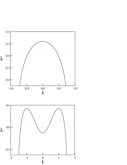
FIG. 1.:

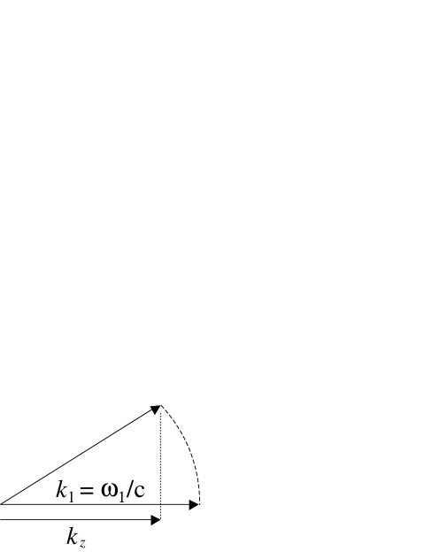
FIG. 2.:

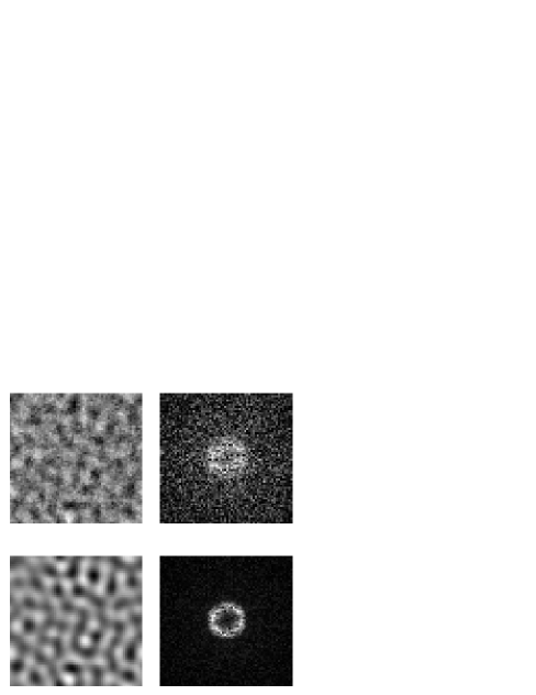
FIG. 3.:

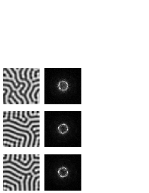
FIG. 4.:

REFERENCES

- [1] M.C. Cross and P.C. Hohenberg, Rev. Mod. Phys. 65, 851 (1993).
- [2] I. Prigogine and G. Nicolis, J. Chem. Phys. 46, 3542 (1967).
- [3] L.A. Ostrovsky and I.A. Soustova, Sov. Phys. Acoust. 22, 416 (1976).
- [4] F.T. Arecchi, S. Bocaletti and P-L. Ramazza, Phys. Rep. 318, 1 (1999).
- [5] F.V. Bunkin, Yu. A. Kravtsov and G.A. Lyskhov, Sov. Phys. Usp. 29, 607 (1986).
- [6] J.W. Miles, J. Fluid. Mech. 146, 285 (1984).
- [7] F. Melo, P. Umbanhowar and H.L. Swinney, Phys. Rev. Lett. 72, 172 (1994).
- [8] V. L’vov, Wave Turbulence Under Parametric Excitation (Springer-Verlag, Berlin, 1994).
- [9] G-L. Oppo, M. Brambilla and L.A. Lugiato, Phys. Rev. A 49, 2028 (1994).
- [10] G. J. de Valcárcel, K. Staliunas, E. Roldán and V.J. Sánchez-Morcillo, Phys. Rev. A 54, 1609 (1996).
- [11] A. Korpel and R. Adler, Appl. Phys. Lett. 7, 106 (1965).
- [12] L. Adler and M.A. Breazeale, J. Acoust. Soc. Am. 48, 1077 (1970).
- [13] N.Yen, J. Acoust. Soc. Am. 57, 1357 (1975).
- [14] L.A. Ostrovsky, I.A. Soustova and A.M. Sutin,Acustica 39, 298 (1978).
- [15] M.F. Hamilton and J.A. TenCate, J. Acoust. Soc. Am. 81, 1703 (1987).
- [16] D. Rinberg, V. Cherepanov and V. Steinberg, Phys. Rev. Lett. 76, 2105 (1996).
- [17] D. Rinberg and V. Steinberg, Phys. Rev. B 64, 054506 (2001).
- [18] M.F. Hamilton and D. Blackstock, Nonlinear Acoustics, Academic Press (1997)
- [19] L.K. Zarembo and O.Y. Serdoboloskaya, Akust.Zh. 20, 726 (1974).
- [20] O.A. Druzhinin, L.A. Ostrovsky and A. Prosperetti, J. Acoust. Soc. Am. 100, 3570 (1996).
- [21] L.A. Ostrovsky, A.M. Sutin, I.A. Soustova, A.I. Matveyev and A.I. Potapov, J. Acoust. Soc. Am. 104, 722 (1998).
- [22] L.A. Lugiato and L M. Narducci, Z. Phys. B -Condensed Matter 71, 129 (1988).
- [23] L.A. Lugiato and C. Oldano, Phys. Rev. A 37, 3896 (1988).
- [24] I. Akhatov, U. Parlizt and W. Lauterborn, J. Acoust. Soc. Am. 96, 3627 (1994).
- [25] I. Akhatov, U. Parlizt and W. Lauterborn, Phys. Rev. E. 54, 4990 (1996).
- [26] O.V. Rudenko, Sov. Phys. Usp. 38, 965 (1995).