Quantum Manifestations of Classical Stochasticity
in the Mixed State

Abstract

We investigate the QMCS in structure of the eigenfunctions, corresponding to mixed type classical dynamics in smooth potential of the surface quadrupole oscillations of a charged liquid drop. Regions of different regimes of classical motion are strictly separated in the configuration space, allowing direct observation of the correlations between the wave function structure and type of the classical motion by comparison of the parts of the eigenfunction, corresponding to different local minima.

1 Introduction

The deformation potential

$$U(a_{0},a_{2})=\sum_{m,n}C_{mn}(a_{0}^{2}+2a_{2}^{2})^{m}a_{0}^{n}(6a_{2}^{2}-a_{0}^{2})^{n}$$ (1)

where $a_{0}$ and $a_{2}$ are the internal coordinates of the drop surface

$$R(\theta,\varphi)=R_{0}\{1+a_{0}Y_{2,0}(\theta,\varphi)+a_{2}[Y_{2,2}(\theta,\varphi)+Y_{2,-2}(\theta,\varphi)]\}$$ (2)

Figure 1: The potential shape for $W=18$.

describes surface quadrupole oscillations of a charged liquid drop of any nature, including atomic nuclei[1] and metal clusters,[2] containing specific character of the interaction only in the coefficients $C_{mn}$. Expanding (1) to fourth order in deformation variables

$$x=\frac{\sqrt{2}C_{20}}{3C_{01}}a_{0},y=\frac{\sqrt{2}C_{20}}{3C_{01}}a_{2}$$ (3)

and assuming equality of masses for the two independent directions, we get the one-parametric $C_{3v}$-symmetric Hamiltonian

$$H=\frac{p_{x}^{2}+p_{y}^{2}}{2m}+U(x,y,W)$$ (4)

$$U(x,y,W)=\frac{1}{2W}(x^{2}+y^{2})+xy^{2}-\frac{1}{3}x^{3}+(x^{2}+y^{2})^{2}$$ (5)

where $W=9C_{01}^{2}/(C_{10}C_{20})$.
The potential (5) is a generalization of the well-known Henon-Heiles potential[3] with one important difference: motion in (5) is finite for all energies, assuring existence of the stationary states in quantum case. For $W>16$ the potential energy surface has seven critical points: four minima (one central and three peripheral) and three saddles. We consider in detail the case $W=18$, when all four minima have the same depth $E=0$ and the saddle energies are $E_{S}=1/20736$. Critical energy of transition to chaos equals $E_{S}$ for the peripheral and roughly $E_{S}/2$ for the central minimum, so we will be interested in the energy range $E_{S}/2<E<E_{S}$, where the classical motion is chaotic in the central and purely regular in peripheral minima, resulting in what we shall call the mixed state.[4, 5]
We find numerically the spectrum $E_{n}$ and the eigenfunctions $\psi_{n}(x,y)$ for the Hamiltonian (4) by the spectral method,[6, 7] which implies the numerical solution of the time-dependent Schrödinger equation

$$i\frac{\partial\psi(x,y,t)}{\partial t}=\left[-\frac{\partial_{x}^{2}+\partial_{y}^{2}}{2m}+U(x,y,W)\right]\psi(x,y,t)$$ (6)

with the symmetrically split operator algorithm[8]

$$\psi(x,y,t+\Delta t)=e^{i\frac{\Delta t\nabla^{2}}{4m}}e^{-i\Delta tU(x,y,W)}e^{i\frac{\Delta t\nabla^{2}}{4m}}\psi(x,y,t)+O(\Delta t^{3})$$ (7)

where $\exp{(i\Delta t\nabla^{2}/4m)}\psi(x,y,t)$ is efficiently calculated using the fast Fourier transform. Initial wave function

$$\psi(x,y,t=0)=\sum_{n}a_{n}\psi_{n}(x,y)$$ (8)

is chosen to assure the convergence of $\psi(x,y,t)$ in both the coordinate and reciprocal spaces and to avoid the degenerate states in the decomposition (8).
Having calculated $\psi(x,y,t)$ for $0<t<T$, we obtain the spectrum $E_{n}$ as the local maxima of

$$P(E)=\frac{1}{T}\int\limits_{0}^{T}dte^{iEt}P(t)w(t)=\sum_{n}|a_{n}|^{2}\delta_{T}(E-E_{n})$$ (9)

and the eigenfunctions $\psi_{n}(x,y)$ as

$$\psi_{n}(x,y)=\frac{1}{T}\int\limits_{0}^{T}dt\psi(x,y,t)w(t)e^{iE_{n}t}$$ (10)

where

$$P(t)=\int dxdy\psi^{*}(x,y,t=0)\psi(x,y,t)$$ (11)

$$\delta_{T}(E-E_{n})=\frac{1}{T}\int\limits_{0}^{T}dtw(t)e^{i(E-E_{n})t}$$ (12)

and $w(t)=1-\cos(2\pi t/T)$ is the Hanning window function.

2 QMCS in the eigenfunction structure

Quantum manifestations of classical stochasticity can be expected in the form of some peculiarities of concrete stationary state[9]cv60 or in the whole group of states close in energy.[12]cv89 Of course, it is not excepted that such alternative does not exist at all, i.e. the manifestations of the classical chaos can be observed both in the properties of separate states and in their sets. For example, comparing the eigenfunctions, corresponding to energy levels below the critical energy of transition to chaos $E_{c}$, with those corresponding to energy levels above $E_{c}$, drastic changes in the eigenfunction structure can be easily seen and analyzed. However, a question can arise if those changes are due to change in the type of classical motion or they are just a result of the quantum numbers change. Instead of comparing the eigenfunctions corresponding to different states, we propose to look for QMCS in the single quantum mechanical object — the eigenfunction of the mixed state.
$C_{3v}$-symmetric Hamiltonian (4) is invariant under rotation of $2\pi/3$ in the $(x,y)$ plain and under reflection through $x$ axis, so according to the transformation properties

$$\psi(r,\varphi+2\pi/3)=R\psi(r,\varphi)$$ (13)

$$\psi(r,-\varphi)=\sigma\psi(r,\varphi)$$ (14)

the eigenfunctions can be divided into three types of different symmetry: $A_{1}(R=1,\sigma=1)$, $A_{2}(R=1,\sigma=-1)$, and double degenerate $E(R=\exp{(\pm 2\pi/3)},\sigma=\pm 1)$. The initial wave function (8) was chosen to excite only $A_{1}$-type states, and we computed the energy levels and the eigenfunctions for (4) with $W=18$ and $m=10^{10}$, which corresponds to the main quantum numbers of order $10^{2}$ in the energy range $E_{S}/2<E<E_{S}$. Computations were made on a $1024\times 1024$ grid of length $0.6$ (distance from the central minimum to saddles was $1/12$ and $1/6$ to the peripheral minima), number of time steps was 16384 with increment $\Delta t=10^{4}$.
Isolines of probability density and nodal curves for the eigenfunction corresponding to $E_{n}=0.444\times 10^{-4}=0.92E_{S}$ are presented in Fig.3,3.

Figure 2: The eigenfunction shape

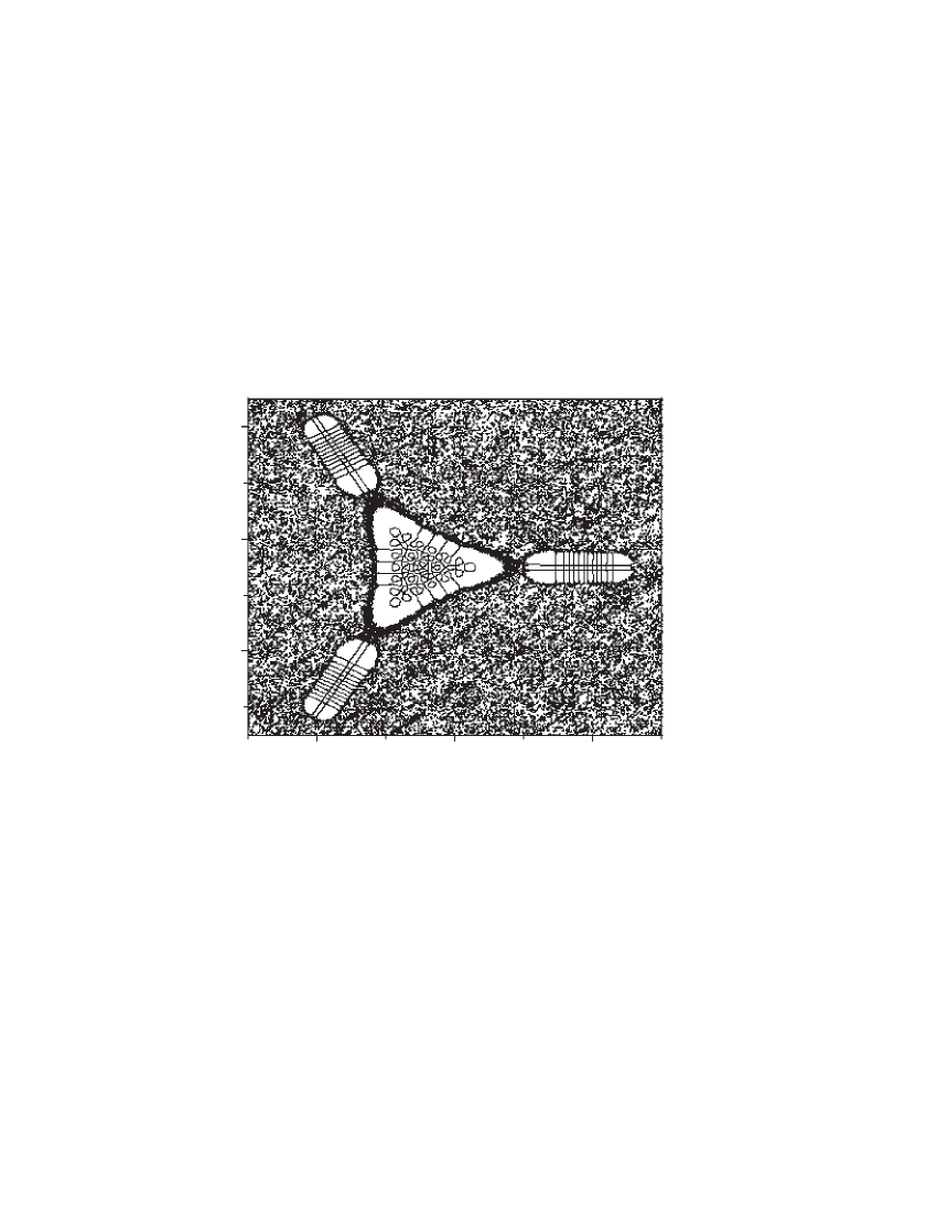
Figure 3: The nodal curves

As we did not compute the entire spectrum, we cannot point out the number $n$ exactly, but we estimate it to be about 200. Correlations between the character of classical motion — developed chaos in the central minimum and pure regularity in the peripheral ones — can be easily seen comparing the parts of the eigenfunction corresponding to different local minima.

3 Conclusion

We considered the quantum manifestations of classical stochasticity in the structure of eigenfunction in the coordinate representation, corresponding to the mixed state in the potential of surface quadrupole oscillations of a charged liquid drop. Correlations between character of classical motion and structure of the eigenfunction parts, corresponding to local minima with different type of classical motion, was observed in the shape of the probability density distribution and in the nodal curves structure, which gives direct and natural way to study the QMCS in smooth potentials. Numerical computations were made by the spectral method, which is a promising alternative to the matrix diagonalization method for the potentials with few local minima.

References

- [1] V. Mozel and W.Creiner, \JLZ.Phys.,217,1968,256.
- [2] W. A. Saunders, \PRL64,1990,3046.
- [3] M. Henon and C. Heiles, \JLAstron.J.,69,1964,73.
- [4] Yu. L. Bolotin, V. Yu. Gonchar and E. V. Inopin, \JLYad.Fiz.,45,1987,351.
- [5] V.P. Berezovoy, Yu.L. Bolotin, V.Yu. Gonchar, M.Ya. Granovsky, Quadrupole oscillation as paradigm of the chaotic motion in nuclei, Particles & Nuclei (in press).
- [6] M. D. Feit, J. A. Fleck, Jr., and A. Steiger, \JLJ. Comput. Phys.,47,1982,412.
- [7] M. D. Feit and J. A. Fleck, Jr., \JLJ.Opt.Soc.Amer.,17,1981,1361.
- [8] J. A. Fleck, Jr., J. R. Morris, and M. D. Feit, \JLAppl.Phys.,10,1976,129.
- [9] M. V. Berry and M. Robnik, \JPA19,1986,1365.
- [10] T. Prosen and M. Robnik, \JPA26,1993,5365.
- [11] Baowen Li and M. Robnik, \JPA: Math. Gen. 28,1995,2799.
- [12] M. V. Berry and M. Robnik, \JPA17,1984,2413.
- [13] M. V. Berry and M. Robnik, \JPA19,1986,649.
- [14] M. Robnik and M. V. Berry, \JPA19,1986,669.
- [15] T. Prosen and M. Robnik, \JPA26,1993,2371.
- [16] Baowen Li and M. Robnik, \JPA27,1994,5509.
- [17] T. Prosen and M. Robnik, \JPA27,1994,L459.
- [18] T. Prosen and M. Robnik, \JPA27,1994,8059.
- [19] Baowen Li and M. Robnik, \JPA: Math. Gen. 29,1996,4387.
- [20] M. Robnik, J. Dobnikar and T. Prosen, \JPA: Math. Gen. 32,1999,1427.
- [21] T. Prosen and M. Robnik, \JPA: Math. Gen. 32,1999,1863.