Localized transverse bursts in inclined layer convection

Abstract

We investigate a novel bursting state in inclined layer thermal convection in which convection rolls exhibit intermittent, localized, transverse bursts. With increasing temperature difference, the bursts increase in duration and number while exhibiting a characteristic wavenumber, magnitude, and size. We propose a mechanism which describes the duration of the observed bursting intervals and compare our results to bursting processes in other systems.

Bursting phenomena are a common feature of nonequilibrium systems. Various bursting mechanisms have been described by Knobloch and Moehlis Knobloch and Moehlis (2000) and characterized in terms of their recurrence properties and dynamic range, distinguishing between temporally localized bursts which are spatially global and those which are spatially local. Some examples of the former are the breakdown of spiral vortices in Taylor-Couette flow Coughlin and Marcus (1996); Coughlin et al. (1999), fluctuations in heat transport in binary fluid convection Sullivan and Ahlers (1988); Moehlis and Knobloch (1998), and shear flow turbulence Waleffe (1998); Grossmann (2000). While a dynamical systems approach has been fruitful in the global case, spatially localized bursts remain less understood.

In the Letter, we characterize a recently discovered Daniels et al. (2000) bursting phenomenon in inclined layer convection (ILC) resulting from the presence of both buoyancy and shear instabilities. Two features are intriguing: spatially localized bursts of a characteristic size and the triggering of local disorder within the burst without completely destroying the underlying roll structure (see Fig. 1). Temporally, we observe multiple cycles of transverse modulation, turbulence, and decay within the bursts. Existing theory does not address either the spatial or temporal dynamics.

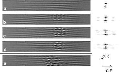
Figure 1: (a–d) Sequence of background-divided shadowgraph images and associated contrast-enhanced power spectra for Cell 1 at $\theta=78^{\circ}$ and $\epsilon=0.08$. (a) quiescent, (b) modulations during early bursting, (c) developed bursting, and (d) end of burstlet. Times correspond to points marked in Fig. 6. Uphill direction is at left. (e) Disordered bursting at $\theta=78^{\circ}$ and $\epsilon=0.09$. Also see movies at EPA .

Inclined layer convection is a variant of Rayleigh-Bénard (thermal) convection Bodenschatz et al. (2000), in which a fluid layer is heated from one side and and cooled from the other. Tilting this layer by an angle $\theta$ (see Fig. 2) results in a base state which is a superposition of a linear temperature gradient and a shear flow up along the hot plate and down along the cold. When heated beyond a critical temperature difference $\Delta T_{c}$, the fluid convects due to the buoyancy of the hot fluid. As $\theta$ is increased, the buoyancy provided by the perpendicular component of gravity $g_{\perp}\equiv g\cos\theta$ becomes weaker and the shear flow provided by $g_{\parallel}$ becomes stronger. Above a codimension-two point at $\theta_{c}$, the primary instability is due to this shear flow instead of buoyancy Hart (1971); Clever and Busse (1977); Fujimura and Kelly (1993). Interesting bursting behavior has been observed in the vicinity of this codimension-two point Daniels et al. (2000).

Figure 2: Schematic diagram of inclined layer convection profile.

We perform experiments in high pressure CO₂ in an apparatus similar to that described in de Bruyn et al. (1996), modified to allow for inclination. The gas was at a pressure of $(48.26\pm 0.01)$ bar regulated to $\pm 0.005$ bar with a mean temperature of $(25.00\pm 0.05)^{\circ}$C regulated to $\pm 0.3$mK. Our three convection cells were of height $d=778\pm 2\mu$m and length $97.3d$. The widths in the $\hat{\bf x}$ direction are $L_{1}=10.4d$ for Cell 1, $L_{2}=20.9d$ for Cell 2, and $L_{3}=31.0d$ for Cell 3. These parameters give a vertical viscous diffusion time of $\tau_{v}=d^{2}/\nu=(4.50\pm 0.02)$ sec, a Prandtl number $\sigma=1.301\pm 0.001$, and weakly non-Boussinesq conditions ($Q=0.2$ to 0.8, as described in Bodenschatz et al. (2000) for horizontal fluid layers). The planform of the convection pattern was observed via the shadowgraph technique de Bruyn et al. (1996) using a digital camera. The two control parameters are the angle $\theta$ and the nondimensionalized temperature difference $\epsilon\equiv{\Delta T\over\Delta T_{c}}-1$. Images were collected at 27 frames/$\tau_{v}$ with runs of duration at least 1000 $\tau_{v}$ at various values of $\epsilon$, $\theta$.

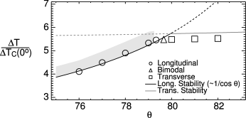
Figure 3: Phase diagram near the codimension-two point of ILC, for Prandtl number $\sigma=1.301$. Stability curves are from Pes ; solid lines are primary instabilities and dashed lines are extensions. Shaded area corresponds to data collection on bursts.

Fig. 3 shows the phase diagram for ILC in the vicinity of the codimension-two point, with onset measured experimentally (data points) and compared to predictions from linear stability analysis Pes . The localized transverse bursts appear intermittently within the underlying longitudinal rolls as a secondary instability for $\theta<\theta_{c}$. These bursts are triggered within a secondary instability in which there is already local growth of regions of high-amplitude longitudinal convection, as seen in the sequence of images in Fig. 1; a movie of the corresponding images are available online EPA . Within these regions, transverse modulations repeatedly grow and decay, becoming disordered or turbulent in the process. Eventually, this cycle of bursting ends and the system returns to quiescent, weak longitudinal rolls. The phenomenon becomes more pronounced at large $\epsilon$, so that eventually the whole cell is bursting. Each localized patch does not spread and no global bursting was observed. At lower inclination (further from the codimension-two point), the bursting is indistinguishable from the crawling rolls described in Daniels et al. (2000).

Figure 4: Wavenumber of transverse bursts $p$ (determined from power spectra) as a function of $\theta$, $\epsilon$, and $L$. In each graph the data plotted are averaged over the other two variables. Dashed lines are $p_{c}/2$ for $\theta=80^{\circ}$.

The measured wavenumber $p$ of the transverse modulations is shown in Fig. 4 and observed to be approximately constant. At $\theta=80^{\circ}$, the transverse rolls were determined to have a wavenumber of $p_{c}=(2.82\pm 0.04)d$ at onset; the burst wavenumber $p$ is nearly subharmonic with respect to this value. The appearance of this bursting phenomena close to the stability curve for transverse rolls suggests that a related shear instability is playing a role. Nonetheless, no mode resonant with $p_{c}$ is observed as part of the bursting spectrum (see Fig. 1).

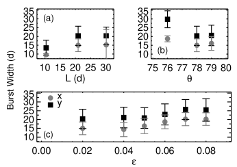
Figure 5: Burst width in $\hat{\bf x}$ (gray) and $\hat{\bf y}$ (black) directions: (a) vs. $L$ at onset of bursting for $\theta=78^{\circ}$, (b) vs. $\theta$ at onset of bursting in Cell 2, and (c) vs. $\epsilon$ in Cell 2 at $\theta=78^{\circ}$.

Using Fourier decomposition, we determined the area of each cell occupied by transverse bursting and found the width of the region for those instances in which only a single burst was present. As shown in Fig. 5, the bursts generally have a characteristic of size of $15d$ in the transverse direction and $20d$ in the longitudinal. Bursts are smaller in Cell 1 (see Fig. 5a), where they fill the cell in the $\hat{\bf x}$ (transverse) direction, and larger for $\theta=76^{\circ}$ (Fig. 5b) and increased $\epsilon$ (Fig. 5c) Cell 2 and Cell 3 typically contain multiple bursts; therefore, we will utilize data from Cell 1 to focus on the temporal behavior of single bursts. For Cells 1, 2, and 3 the onset of bursting was observed to occur at $\epsilon=0.075$, $\epsilon=0.02$, and $\epsilon=0.04$, respectively ons .

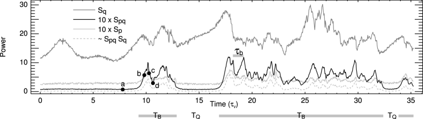
Figure 6: Sample segments of $S_{q}(t)$, $S_{pq}(t)$, and $S_{p}(t)$ at $\epsilon=0.08$ and $\theta=78^{\circ}$ in Cell 1. Power is in arbitrary units. Labeled black dots correspond to the images in Fig. 1. Gray bars indicated bursting; time intervals $T_{B}$, $T_{Q}$, and $\tau_{b}$ defined in text.

   

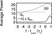
Figure 7: (a) Cross-correlation of ($S_{pq}$, $S_{q}$), dashed and ($S_{pq}$, $S_{p}$), solid. (b) Ensemble average $\langle S(t-t_{\mathrm{s}tart})\rangle$ over all bursts where $t_{\mathrm{s}tart}$ is the rising edge of $S_{pq}$ for each burst. Both are plotted for Cell 1 at $\epsilon=0.08$ and $\theta=78^{\circ}$. Power is in same arbitrary units as Fig. 6.

We describe the bursts based on the modes they excite in Fourier space, using the power spectra of background-divided images as a function of time. Sample spectra and their corresponding shadowgraph images are shown in Fig. 1, with three prominent modes: a pure $\hat{\bf x}$ mode $q$, a pure $\hat{\bf y}$ mode $p$, and a mixed mode $pq$. The longitudinal rolls are composed of the pure $q$ mode, while the transverse modulations are constructed from the $p$ and $pq$ modes. Higher-order modes serve to create the characteristic shape of the bursts and will be ignored here. A further simplification should be noted: the shadowgraph technique integrates through the fluid layer ($\hat{\bf z}$), while these bursting phenomena exhibit three dimensional behavior, particularly when the modulations become disordered.

We define $S_{q}$, $S_{pq}$, and $S_{p}$ as the power in each of these three peaks, taken as the total intensity in a fixed region of Fourier space. Fig. 6 shows time traces of the power in each of the three modes. Prior to the beginning of the burst $S_{q}$ typically increases in relative amplitude, as shown in Fig. 7a. The beginning of a burst is characterized by the rapid growth of the transverse modulations (via $S_{pq}$). The $S_{p}$ mode is weaker and grows after a delay of about $0.5\tau_{v}$ (see Fig. 7b), which suggests that it is due to a nonlinear interaction or resonance condition between the $q$ and $pq$ modes. The simplest such nonlinearity would be quadratic, and by multiplying $S_{q}(t)$ and $S_{pq}(t)$, we obtain a good reproduction of the curve for $S_{p}(t)$, shown as the gray dashed line in Fig. 6.

The time series in Fig. 6 show two temporal features: (1) intermittent, alternating periods of quiescence and bursting and (2) burstlets characterized by peaks and troughs within the bursting intervals. As $S_{pq}(t)$ rises at the beginning of a burstlet, the pattern exhibits the increasingly well-defined modulations shown in Fig. 1b. When $S_{pq}$ peaks, these modulations become spatially disordered on short time scales, moving rapidly within the underlying rolls. While the general roll pattern is retained in any single image (see Fig. 1c), the roll segments move turbulently within the localized bursting region EPA . At higher $\epsilon$ and $\theta$, both of which increase the shear flow, this disorder is increased (see Fig. 1d). From the disordered state, the modulations either decay — resulting in the end of the bursting interval — or grow again, creating another burstlet within the same interval. A succession of such events is suggestive of the presence of a limit cycle. Stochastic limit cycles have been previously described in Knobloch and Moehlis (2000); Busse (1984), relying on a random forcing effect such as pressure fluctuations to produce random events with a single, well-defined mean rate.

To determine the quiescent and bursting intervals, we set a threshold for $S_{pq}(t)$ above which the system was considered to be bursting. Because the onset and decay of the burst is sharp, the results were not sensitive to the choice of threshold over a reasonable range of values. Using this information, we examined the duration of quiescent intervals $T_{Q}$, bursting intervals $T_{B}$. Burstlets are separated by intervals $\tau_{b}$ within the $T_{B}$, with burstlet peaks identified by local maximum. Examples of the determined bursting intervals are shown by the gray bars at the bottom of Fig. 6. Sample probability distribution functions (PDFs) and mean values as a function of $\epsilon$ are plotted in Fig. 8. The quiescent intervals $T_{Q}$ were longest close to the onset of bursting, and decreased until they were no longer detectable at higher $\epsilon$. Conversely, the bursting intervals $T_{B}$ grow with $\epsilon$. The combined effect is that at high $\epsilon$ the whole cell is in a perpetual state of bursting since each localized burst lives longer and new ones begin sooner. All of these trends hold at other values of $\epsilon$ and $\theta$ as well.

Such behavior distinguishes this bursting from the behavior of bursts in Taylor-Couette flow Coughlin and Marcus (1996); Coughlin et al. (1999). There, the bursting is attributed to a secondary instability whose growth above a threshold triggers turbulence throughout the fluid. Once the turbulence has begun it destroys the underlying rolls which were providing energy and thus it dies away after a well-defined period of time. It appears that the initial transverse modulations in ILC are such a secondary instability, although they appear to arise due to a growing primary mode which triggers their onset, as shown in Fig. 7. However, instead of fully bursting, the burstlets cause only local disorder and fail to globally trigger turbulence. Because the modulation and rolls are not completely destroyed (see Fig. 6), they are readily able to grow back up again after they decay. This creates bursts comprised of multiple burstlets. As a result, $T_{B}$ is not constant as was observed for the Taylor-Couette bursts but instead increases with $\epsilon$, as shown in Fig. 8f. The mechanism for the growth of the Taylor-Couette bursts Coughlin and Marcus (1996); Coughlin et al. (1999) provides for $\langle T_{Q}\rangle\sim 1/\epsilon$ behavior based on a constant growth rate of the secondary instability. It is possible that a similar mechanism is at work since a similar trend of longer quiescent periods at lower $\epsilon$ is observed (see Fig. 8d.)

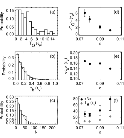
Figure 8: (a,b,c) Sample PDFs of $T_{Q}$, $\tau_{b}$, and $N$ respectively at $\epsilon=0.08$ and $\theta=78^{\circ}$. (b) Dashed line is exponential distribution fit to data excluding the first bin. (c) Dashed line is Eqn. 3 plotted from the measured mean. (d) Mean quiescent period as a function of $\epsilon$ at $\theta=78^{\circ}$. (e) Measured and effective (from fit) mean burstlet period and (f) mean number of burstlets and mean bursting interval as a function of $\epsilon$ at $\theta=78^{\circ}$.

To create cycles of burstlets within each bursting interval, a second bursting process must be at work as well. At each $\epsilon$ and $\theta$ the PDF of $\tau_{b}$ (see Fig. 8b) exhibits a negative exponential distribution

$${\cal P}(\tau_{b})={e^{-\tau_{b}/\langle\tau_{b}\rangle}\over{\langle\tau_{b}\rangle}}$$ (1)

where $\langle\tau_{b}\rangle$ is the mean waiting period of a Poisson process generating the bursts. Because the lowest $\tau_{b}$ bin is underreported due to the finite sampling of the time series, $\langle\tau_{b}\rangle_{\mathrm{e}ff}$ is found instead by fitting the negative exponential to all data except for the first bin.

This description can also explain why $T_{B}$ isn’t constant. In a Poisson process, the events are memoryless: the wait time for the next event is independent of how long the system has already been waiting. If a new burstlet were not generated before the decay to quiescence, the modulations would die away and the burst interval would be over. Assuming a constant, unknown decay time $\tau_{d}$, the probability distribution for $N$ burstlets for which each $\tau_{b}$ is no more than $\tau_{d}$ is calculated using the cumulative distribution of Eqn. 1, ${\cal P}(\tau_{b}\leq\tau_{d})=1-e^{-\tau_{b}/\tau_{d}}$.

$${\cal P}(N)={(1-{e}^{-\tau_{d}/\langle\tau_{b}\rangle})^{N}\over{e}^{\tau_{d}/\langle\tau_{b}\rangle}-1}$$ (2)

This distribution contains a single parameter $\langle N\rangle\equiv{e}^{\tau_{d}/\langle\tau_{b}\rangle}$, which can be measured directly from the experimental ${\cal P}(N)$. Eqn. 2 then reduces to

$${\cal P}(N)={(\langle N\rangle-1)^{N-1}\over\langle N\rangle^{N}}$$ (3)

where $\langle N\rangle$ is the measured mean number of burstlets per interval. This formulation allows for comparison with the observed data with no fit parameters. Fig. 8c shows good agreement with this model, as do plots at other parameter values. Therefore, our results are consistent with the burstlets being Poisson-distributed events.

Transverse bursts in inclined layer convection show many consistent and unexplained properties across a range of $\epsilon$ and $\theta$: spatial localization, transverse modulations of uniform wavenumber, persistence of the roll structure while bursting, and repeated cycles of growth and decay once triggered. Aspects of both spatiotemporal chaos and turbulence appear to be relevant and these results represent a first step in understanding the structure and dynamics of this novel bursting phenomenon. In particular, more work is needed to understand both the local growth of longitudinal rolls which triggers the bursting and the implications of a resonance condition between the $p$, $q$, and $pq$ modes.

We wish to thank W. Pesch and J. Brink for sharing results from stability analysis and full numerical simulations and J. P. Sethna for fruitful discussions. We are grateful to NSF for support under DMR-0072077 and the IGERT program in nonlinear systems, DGE-9870631.

References

- Knobloch and Moehlis (2000) E. Knobloch and J. Moehlis, in Nonlinear Instability, Chaos and Turbulence, Vol. II, edited by L. Debnath and D. Riahi (Computational Mechanics Publications, Southampton, 2000), pp. 237–87.
- Coughlin and Marcus (1996) K. Coughlin and P. S. Marcus, Phys. Rev. Lett. 77, 2214 (1996).
- Coughlin et al. (1999) K. Coughlin, C. F. Hamill, P. S. Marcus, and H. L. Swinney (1999), preprint.
- Sullivan and Ahlers (1988) T. S. Sullivan and G. Ahlers, Phys. Rev. A 38, 3143 (1988).
- Moehlis and Knobloch (1998) J. Moehlis and E. Knobloch, Phys. Rev. Lett. 80, 5329 (1998).
- Waleffe (1998) F. Waleffe, Phys. Rev. Lett. 81, 4140 (1998).
- Grossmann (2000) S. Grossmann, Rev. Mod. Phys. 72, 603 (2000).
- Daniels et al. (2000) K. E. Daniels, B. B. Plapp, and E. Bodenschatz, Phys. Rev. Lett. 84, 5320 (2000).
- (9) Movies of bursting behavior are available at EPAPS.
- Bodenschatz et al. (2000) E. Bodenschatz, W. Pesch, and G. Ahlers, Ann. Rev. of Fluid Mech. 32, 709 (2000).
- Hart (1971) J. E. Hart, J. Fluid Mech. 47, 547 (1971).
- Clever and Busse (1977) R. M. Clever and F. H. Busse, J. of Fluid Mech. 81, 107 (1977).
- Fujimura and Kelly (1993) K. Fujimura and R. E. Kelly, J. Fluid Mech. 246, 545 (1993).
- de Bruyn et al. (1996) J. R. de Bruyn, E. Bodenschatz, S. W. Morris, S. P. Trainoff, Y. Hu, D. S. Cannell, and G. Ahlers, Rev. of Sci. Inst. 67, 2043 (1996).
- (15) W. Pesch, private communication.
- (16) In addition to different onsets, the three cells were also observed to have somewhat different burst strengths, with Cell 2 exhibiting the strongest bursts. These effects may be related to a resonance between the width of the cells and , to finite-size effects, or to temperature inhomogeneities.
- Busse (1984) F. H. Busse, in Turbulence and Chaotic Phenomena in Fluids, edited by T. Tatsumi (Amsterdam, 1984), ISBN 0444875948.